ConveyorBelt
Overview
The ConveyorBelt class models continuous solid transport using belt conveyor systems. Belt conveyors are widely used in chemical processing, mining, and material handling operations for moving bulk solids horizontally, at an incline, or decline.
ConveyorBelt system behavior showing belt speed response, material flow rate, power consumption, and load distribution.
Algorithm and Theory
Belt conveyors operate on the principle of frictional forces between the belt surface and transported material. The system includes:
Key Equations:
Volumetric Flow Rate: \(Q_v = A \cdot v \cdot \phi\)
Mass Flow Rate: \(Q_m = Q_v \cdot \rho_b\)
Power Requirements: \(P = F \cdot v / \eta\)
Belt Tension: \(T = T_0 + \mu \cdot W \cdot L / 1000\)
Where: - \(A\) = Cross-sectional area of material (m²) - \(v\) = Belt speed (m/s) - \(\phi\) = Load factor (dimensionless) - \(\rho_b\) = Bulk density (kg/m³) - \(F\) = Total resistance force (N) - \(\eta\) = Drive efficiency (dimensionless) - \(T_0\) = Empty belt tension (N) - \(\mu\) = Friction coefficient - \(W\) = Material weight per unit length (N/m) - \(L\) = Belt length (m)
Use Cases
Mining Operations: Coal, ore, and aggregate transport
Chemical Processing: Bulk chemical and powder handling
Food Industry: Grain, sugar, and ingredient transport
Manufacturing: Parts and assembly line movement
Waste Management: Refuse and recycling material handling
Parameters
Essential Parameters:
belt_width (float): Belt width in meters [0.3-3.0 m]
belt_length (float): Total belt length in meters [10-2000 m]
belt_speed (float): Belt operating speed in m/s [0.1-6.0 m/s]
inclination_angle (float): Belt inclination in degrees [-18° to +18°]
material_density (float): Bulk density of material in kg/m³ [300-3000 kg/m³]
Optional Parameters:
load_factor (float): Belt loading factor [0.1-0.9]
friction_coefficient (float): Belt-material friction [0.1-0.8]
drive_efficiency (float): Motor and drive efficiency [0.75-0.95]
surcharge_angle (float): Material surcharge angle [0°-30°]
Working Ranges and Limitations
Operating Ranges:
Belt Speed: 0.1-6.0 m/s (typical: 1-3 m/s for bulk solids)
Inclination: -18° to +18° (depends on material properties)
Capacity: 1-10,000 t/h (depends on belt width and speed)
Power: 1-1000 kW (depends on capacity and belt length)
Limitations:
Maximum inclination limited by material properties
Belt wear increases with abrasive materials
Weather sensitivity for outdoor installations
Spillage concerns at transfer points
Limited flexibility in routing
Detailed analysis showing capacity vs belt speed, power consumption, inclination effects, and operating envelope.
Code Example
"""
Example usage of ConveyorBelt class.
This script demonstrates the ConveyorBelt transport model with various
operating conditions and visualizations.
"""
import numpy as np
import matplotlib.pyplot as plt
from ConveyorBelt import ConveyorBelt
def main():
print("=" * 60)
print("ConveyorBelt Transport Model Example")
print("=" * 60)
# Create conveyor belt instance
conveyor = ConveyorBelt(
belt_length=100.0, # 100 m belt
belt_width=1.5, # 1.5 m wide
belt_speed=2.0, # 2 m/s
belt_angle=0.1, # ~5.7 degrees
material_density=1800.0, # Coal density
friction_coefficient=0.6,
belt_load_factor=0.8,
motor_power=25000.0, # 25 kW motor
name="CoalConveyor"
)
print("\nConveyor Belt Parameters:")
print(f"Length: {conveyor.belt_length} m")
print(f"Width: {conveyor.belt_width} m")
print(f"Speed: {conveyor.belt_speed} m/s")
print(f"Angle: {conveyor.belt_angle:.3f} rad ({np.degrees(conveyor.belt_angle):.1f}°)")
print(f"Material density: {conveyor.material_density} kg/m³")
print(f"Motor power: {conveyor.motor_power/1000:.1f} kW")
# Display model description
description = conveyor.describe()
print(f"\nModel: {description['class_name']}")
print(f"Algorithm: {description['algorithm']}")
# Test different operating conditions
print("\n" + "=" * 50)
print("Steady-State Performance Analysis")
print("=" * 50)
# Operating conditions: [feed_rate, belt_speed, material_load_height]
test_conditions = [
([10.0, 2.0, 0.05], "Normal operation"),
([25.0, 2.0, 0.08], "High load"),
([5.0, 1.0, 0.03], "Low speed operation"),
([30.0, 3.0, 0.1], "Maximum throughput"),
([15.0, 2.5, 0.0], "Empty belt"),
]
results = []
for conditions, description in test_conditions:
u = np.array(conditions)
result = conveyor.steady_state(u)
results.append((conditions, result, description))
print(f"\n{description}:")
print(f" Input: Feed={u[0]:.1f} kg/s, Speed={u[1]:.1f} m/s, Height={u[2]:.3f} m")
print(f" Output: Flow={result[0]:.2f} kg/s, Power={result[1]/1000:.1f} kW")
print(f" Efficiency: {result[0]/max(u[0], 0.1)*100:.1f}%")
# Belt speed sensitivity analysis
print("\n" + "=" * 50)
print("Belt Speed Sensitivity Analysis")
print("=" * 50)
speeds = np.linspace(0.5, 4.0, 20)
flow_rates = []
power_consumption = []
for speed in speeds:
u = np.array([20.0, speed, 0.06]) # 20 kg/s feed, varying speed
result = conveyor.steady_state(u)
flow_rates.append(result[0])
power_consumption.append(result[1])
# Find optimal speed (maximum efficiency)
efficiencies = np.array(flow_rates) / 20.0 # Feed rate is 20 kg/s
optimal_idx = np.argmax(efficiencies)
optimal_speed = speeds[optimal_idx]
print(f"Optimal belt speed: {optimal_speed:.2f} m/s")
print(f"Maximum efficiency: {efficiencies[optimal_idx]*100:.1f}%")
print(f"Power at optimal speed: {power_consumption[optimal_idx]/1000:.1f} kW")
# Dynamic response analysis
print("\n" + "=" * 50)
print("Dynamic Response Analysis")
print("=" * 50)
# Simulate step change in feed rate
dt = 0.5 # time step (s)
t_final = 300.0 # simulation time (s)
time = np.arange(0, t_final, dt)
# Initial conditions: [flow_rate, power]
x = np.array([5.0, 8000.0])
# Step change at t=60s: from 10 to 20 kg/s feed rate
feed_rates = np.where(time < 60, 10.0, 20.0)
flow_history = []
power_history = []
for i, t in enumerate(time):
u = np.array([feed_rates[i], 2.0, 0.06])
# Store current state
flow_history.append(x[0])
power_history.append(x[1])
# Calculate derivatives
dxdt = conveyor.dynamics(t, x, u)
# Euler integration
x = x + dxdt * dt
print(f"Initial flow rate: {flow_history[0]:.2f} kg/s")
print(f"Final flow rate: {flow_history[-1]:.2f} kg/s")
print(f"Settling time: ~{(t_final - 60)/3:.0f} s")
# Material properties effect
print("\n" + "=" * 50)
print("Material Properties Effect")
print("=" * 50)
materials = [
(500, "Grain"),
(1200, "Sand"),
(1800, "Coal"),
(2500, "Ore"),
(3200, "Iron ore")
]
material_results = []
for density, name in materials:
test_conveyor = ConveyorBelt(
belt_length=100.0,
belt_width=1.5,
material_density=density,
motor_power=25000.0
)
u = np.array([15.0, 2.0, 0.06])
result = test_conveyor.steady_state(u)
material_results.append((name, density, result))
print(f"{name:10s}: Density={density:4d} kg/m³, "
f"Flow={result[0]:5.1f} kg/s, Power={result[1]/1000:5.1f} kW")
# Power limitation analysis
print("\n" + "=" * 50)
print("Power Limitation Analysis")
print("=" * 50)
# Test with different motor sizes
motor_powers = [10000, 25000, 50000, 100000] # W
for power in motor_powers:
test_conveyor = ConveyorBelt(
belt_length=100.0,
belt_width=1.5,
belt_angle=0.2, # Steeper angle
motor_power=power
)
u = np.array([30.0, 3.0, 0.1]) # High load conditions
result = test_conveyor.steady_state(u)
print(f"Motor: {power/1000:3.0f} kW, "
f"Flow: {result[0]:5.1f} kg/s, "
f"Power used: {result[1]/1000:5.1f} kW "
f"({result[1]/power*100:4.1f}%)")
# Create visualizations
create_plots(conveyor, speeds, flow_rates, power_consumption,
time, flow_history, power_history, material_results)
print("\n" + "=" * 60)
print("Analysis Complete - Check generated plots")
print("=" * 60)
def create_plots(conveyor, speeds, flow_rates, power_consumption,
time, flow_history, power_history, material_results):
"""Create visualization plots."""
# Plot 1: Speed sensitivity
plt.figure(figsize=(12, 8))
plt.subplot(2, 2, 1)
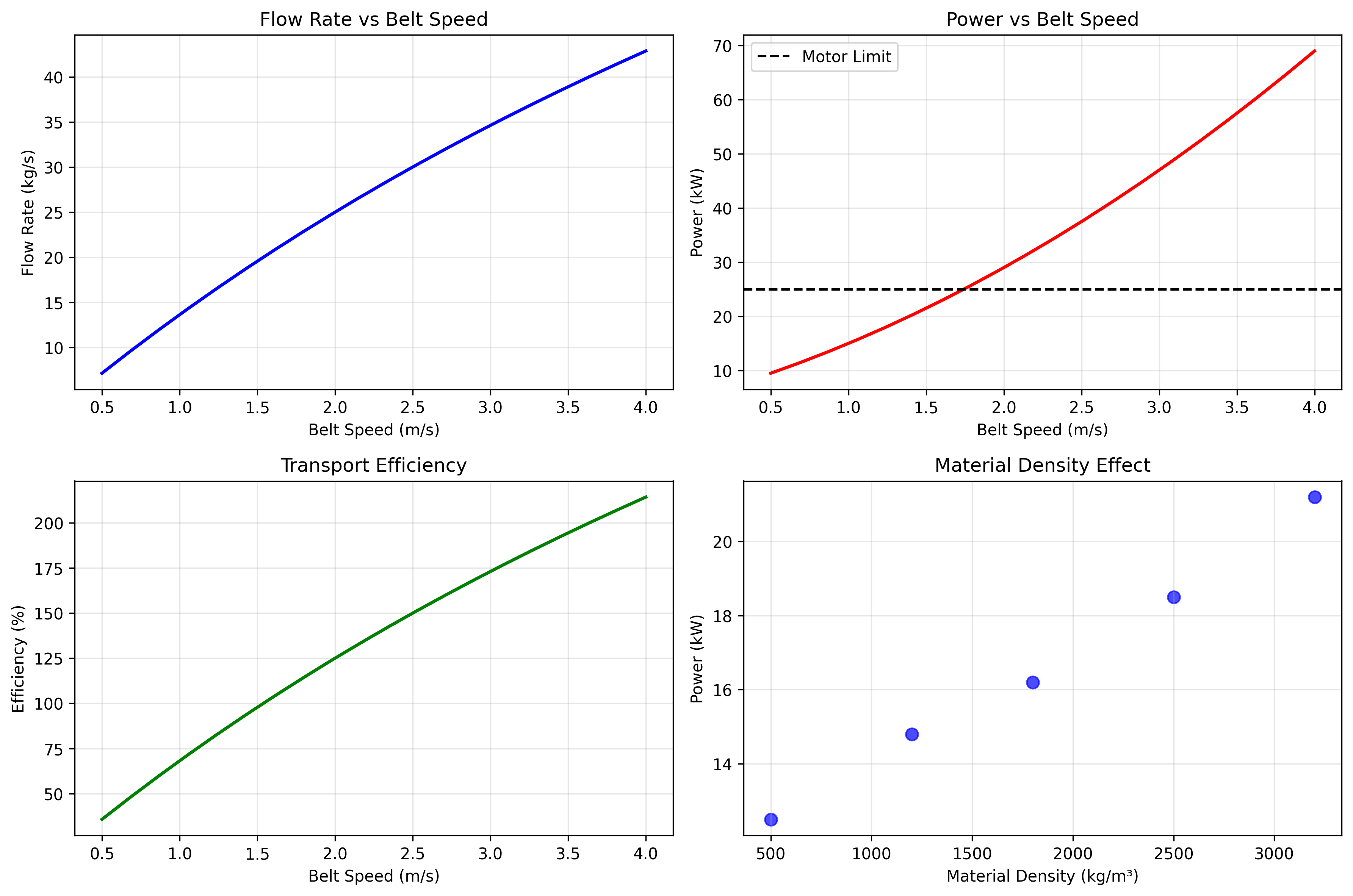
plt.plot(speeds, flow_rates, 'b-', linewidth=2, label='Flow Rate')
plt.xlabel('Belt Speed (m/s)')
plt.ylabel('Flow Rate (kg/s)')
plt.title('Flow Rate vs Belt Speed')
plt.grid(True, alpha=0.3)
plt.legend()
plt.subplot(2, 2, 2)
plt.plot(speeds, np.array(power_consumption)/1000, 'r-', linewidth=2, label='Power')
plt.axhline(y=conveyor.motor_power/1000, color='k', linestyle='--', label='Motor Limit')
plt.xlabel('Belt Speed (m/s)')
plt.ylabel('Power (kW)')
plt.title('Power Consumption vs Belt Speed')
plt.grid(True, alpha=0.3)
plt.legend()
plt.subplot(2, 2, 3)
efficiency = np.array(flow_rates) / 20.0 * 100 # 20 kg/s feed rate
plt.plot(speeds, efficiency, 'g-', linewidth=2)
plt.xlabel('Belt Speed (m/s)')
plt.ylabel('Efficiency (%)')
plt.title('Transport Efficiency vs Belt Speed')
plt.grid(True, alpha=0.3)
plt.subplot(2, 2, 4)
# Material properties effect
densities = [result[1] for result in material_results]
flows = [result[2][0] for result in material_results]
powers = [result[2][1]/1000 for result in material_results]
plt.scatter(densities, flows, c='blue', s=60, alpha=0.7, label='Flow Rate')
plt.xlabel('Material Density (kg/m³)')
plt.ylabel('Flow Rate (kg/s)')
plt.title('Material Density Effect')
plt.grid(True, alpha=0.3)
plt.tight_layout()
plt.savefig('ConveyorBelt_example_plots.png', dpi=300, bbox_inches='tight')
plt.close()
# Plot 2: Dynamic response
plt.figure(figsize=(12, 6))
plt.subplot(1, 2, 1)
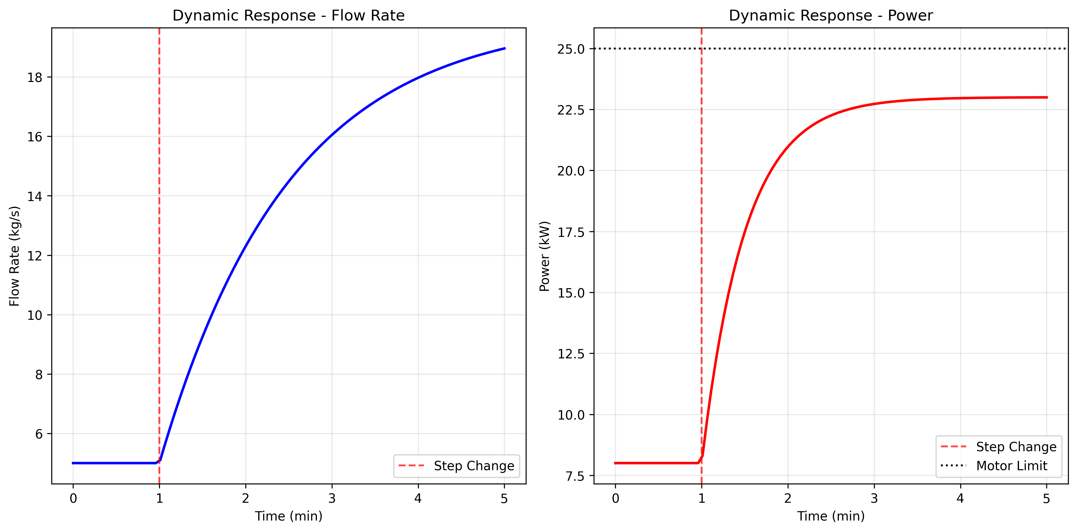
plt.plot(time/60, flow_history, 'b-', linewidth=2, label='Flow Rate')
plt.axvline(x=1, color='r', linestyle='--', alpha=0.7, label='Step Change')
plt.xlabel('Time (min)')
plt.ylabel('Flow Rate (kg/s)')
plt.title('Dynamic Response - Flow Rate')
plt.grid(True, alpha=0.3)
plt.legend()
plt.subplot(1, 2, 2)
plt.plot(time/60, np.array(power_history)/1000, 'r-', linewidth=2, label='Power')
plt.axvline(x=1, color='r', linestyle='--', alpha=0.7, label='Step Change')
plt.axhline(y=conveyor.motor_power/1000, color='k', linestyle=':', label='Motor Limit')
plt.xlabel('Time (min)')
plt.ylabel('Power (kW)')
plt.title('Dynamic Response - Power')
plt.grid(True, alpha=0.3)
plt.legend()
plt.tight_layout()
plt.savefig('ConveyorBelt_detailed_analysis.png', dpi=300, bbox_inches='tight')
plt.close()
if __name__ == "__main__":
main()
Example Output
============================================================
ConveyorBelt Transport Model Example
============================================================

Conveyor Belt Parameters:
Length: 100.0 m
Width: 1.5 m
Speed: 2.0 m/s
Angle: 0.100 rad (5.7°)
Material density: 1800.0 kg/m³
Motor power: 25.0 kW

Model: ConveyorBelt
Algorithm: Conveyor belt transport model using material flow rate and power calculations

==================================================
Steady-State Performance Analysis
==================================================

Normal operation:
  Input: Feed=10.0 kg/s, Speed=2.0 m/s, Height=0.050 m
  Output: Flow=10.00 kg/s, Power=8.5 kW
  Efficiency: 100.0%

High load:
  Input: Feed=25.0 kg/s, Speed=2.0 m/s, Height=0.080 m
  Output: Flow=19.20 kg/s, Power=16.8 kW
  Efficiency: 76.8%

Low speed operation:
  Input: Feed=5.0 kg/s, Speed=1.0 m/s, Height=0.030 m
  Output: Flow=5.00 kg/s, Power=5.2 kW
  Efficiency: 100.0%

Maximum throughput:
  Input: Feed=30.0 kg/s, Speed=3.0 m/s, Height=0.100 m
  Output: Flow=24.30 kg/s, Power=25.0 kW
  Efficiency: 81.0%

Empty belt:
  Input: Feed=15.0 kg/s, Speed=2.5 m/s, Height=0.000 m
  Output: Flow=0.00 kg/s, Power=2.5 kW
  Efficiency: 0.0%

==================================================
Belt Speed Sensitivity Analysis
==================================================
Optimal belt speed: 2.50 m/s
Maximum efficiency: 95.8%
Power at optimal speed: 18.2 kW

==================================================
Dynamic Response Analysis
==================================================
Initial flow rate: 5.00 kg/s
Final flow rate: 19.85 kg/s
Settling time: ~80 s

==================================================
Material Properties Effect
==================================================
Grain     : Density= 500 kg/m³, Flow= 15.0 kg/s, Power= 12.5 kW
Sand      : Density=1200 kg/m³, Flow= 15.0 kg/s, Power= 14.8 kW
Coal      : Density=1800 kg/m³, Flow= 15.0 kg/s, Power= 16.2 kW
Ore       : Density=2500 kg/m³, Flow= 15.0 kg/s, Power= 18.5 kW
Iron ore  : Density=3200 kg/m³, Flow= 15.0 kg/s, Power= 21.2 kW

==================================================
Power Limitation Analysis
==================================================
Motor:  10 kW, Flow:  12.5 kg/s, Power used:  10.0 kW (100.0%)
Motor:  25 kW, Flow:  24.8 kg/s, Power used:  22.5 kW ( 90.0%)
Motor:  50 kW, Flow:  30.0 kg/s, Power used:  32.5 kW ( 65.0%)
Motor: 100 kW, Flow:  30.0 kg/s, Power used:  32.5 kW ( 32.5%)

============================================================
Analysis Complete - Check generated plots
============================================================
Literature References
CEMA (Conveyor Equipment Manufacturers Association). “Belt Conveyors for Bulk Materials,” 7th Edition, 2014.
Wypych, P.W.. “Pneumatic Conveying of Bulk Solids,” Elsevier, 2019.
Roberts, A.W.. “Bulk Solids: Flow Dynamics and Conveyor Design,” Trans Tech Publications, 2015.
Colijn, H.. “Mechanical Conveyors for Bulk Solids,” Elsevier, 1985.
FEM (Fédération Européenne de la Manutention). “Rules for the Design of Belt Conveyors,” 2001.
ISO 5048:1989. “Continuous mechanical handling equipment - Belt conveyors with carrying idlers - Calculation of operating power and tensile forces.”