VacuumTransfer
Vacuum powder transfer model for batch operations (steady-state and dynamic).
Overview
The VacuumTransfer class models pneumatic powder transfer systems using vacuum pumps and cyclone separators. This model is widely used in pharmaceutical, food, and chemical industries for transferring fine powders and granular materials through enclosed piping systems.
Use Case
The vacuum transfer system is employed when:
Fine powder handling requires dust containment
Materials are sensitive to contamination
Transfer over long distances or multiple elevation changes
Automated material handling is required
Clean-in-place (CIP) capabilities are needed
Mathematical Model
Steady-State Model
The steady-state calculation determines transfer rate and vacuum level based on:
Air Flow Calculation: Through transfer line considering pressure drop
Powder Entrainment: Based on air velocity and particle pickup velocity
Cyclone Separation: Efficiency factor for powder collection
System Resistance: Line resistance and filter loading effects
Key equations:
where:
Dynamic Model
The dynamic model tracks:
Powder transfer rate response with entrainment dynamics
Vacuum level response considering pump and system characteristics
First-order time constants for both variables
State equations:
where \(\tau_{\text{transfer}} = 3.0\) s and \(\tau_{\text{vacuum}} = 5.0\) s are the response time constants.
Parameters
Parameter |
Range |
Unit |
Description |
|---|---|---|---|
vacuum_pump_capacity |
10.0 - 500.0 |
m³/h |
Vacuum pump volumetric capacity |
transfer_line_diameter |
0.02 - 0.15 |
m |
Transfer line internal diameter |
transfer_line_length |
1.0 - 100.0 |
m |
Transfer line length |
powder_density |
200.0 - 1500.0 |
kg/m³ |
Powder bulk density |
particle_size |
10e-6 - 500e-6 |
m |
Average particle diameter |
cyclone_efficiency |
0.8 - 0.99 |
Cyclone separator efficiency |
|
vacuum_level_max |
-100000 - 0 |
Pa |
Maximum vacuum level (gauge) |
filter_resistance |
100.0 - 5000.0 |
Pa⋅s/m³ |
Filter pressure drop resistance |
Examples
Basic Usage
from transport.batch.solid.VacuumTransfer import VacuumTransfer
import numpy as np

# Create pharmaceutical vacuum transfer system
pharma_vacuum = VacuumTransfer(
    vacuum_pump_capacity=80.0,      # 80 m³/h pump
    transfer_line_diameter=0.04,    # 40 mm diameter line
    transfer_line_length=12.0,      # 12 m transfer line
    powder_density=500.0,           # Light pharmaceutical powder
    particle_size=50e-6,            # 50 micron particles
    cyclone_efficiency=0.95,        # High efficiency cyclone
    vacuum_level_max=-75000.0,      # -75 kPa max vacuum
    filter_resistance=1500.0        # Higher filter resistance
)

# Steady-state calculation
u = np.array([0.7, -60000.0, 0.3])  # [powder_level, vacuum_setpoint, filter_loading]
result = pharma_vacuum.steady_state(u)
powder_rate, vacuum_level = result
print(f"Powder rate: {powder_rate:.3f} kg/s")
print(f"Vacuum level: {vacuum_level/1000:.1f} kPa")
Particle Size Sensitivity
# Analyze effect of particle size on transfer rate
particle_sizes = np.array([20, 50, 100, 200, 300]) * 1e-6  # microns
transfer_rates = []

for particle_size in particle_sizes:
    # Temporarily modify particle size
    original_size = pharma_vacuum.particle_size
    pharma_vacuum.particle_size = particle_size

    u_test = np.array([0.6, -70000.0, 0.3])
    result = pharma_vacuum.steady_state(u_test)
    transfer_rates.append(result[0])

    # Restore original size
    pharma_vacuum.particle_size = original_size

# Plot results
import matplotlib.pyplot as plt
plt.figure(figsize=(8, 6))
plt.plot(particle_sizes*1e6, transfer_rates, 'o-')
plt.xlabel('Particle Size (μm)')
plt.ylabel('Transfer Rate (kg/s)')
plt.title('Particle Size Effect on Transfer Rate')
plt.grid(True)
plt.show()
Dynamic Simulation
# Dynamic simulation of vacuum system startup
import matplotlib.pyplot as plt

time_span = np.linspace(0, 120, 241)  # 2 minutes
dt = time_span[1] - time_span[0]

# Initial conditions
x = np.array([0.0, 0.0])  # [powder_rate=0, vacuum_level=0]
u = np.array([0.7, -60000.0, 0.2])  # [powder_level, vacuum_setpoint, filter_loading]

# Storage for results
powder_rates = []
vacuum_levels = []

# Euler integration
for t in time_span:
    powder_rates.append(x[0])
    vacuum_levels.append(x[1]/1000)  # Convert to kPa

    # Calculate derivatives
    dx_dt = pharma_vacuum.dynamics(t, x, u)
    # Update state
    x = x + dx_dt * dt

# Plot results
plt.figure(figsize=(10, 8))
plt.subplot(2, 1, 1)
plt.plot(time_span, powder_rates)
plt.ylabel('Powder Rate (kg/s)')
plt.title('VacuumTransfer Dynamic Response')

plt.subplot(2, 1, 2)
plt.plot(time_span, vacuum_levels)
plt.xlabel('Time (s)')
plt.ylabel('Vacuum Level (kPa)')
plt.show()
Filter Loading Analysis
# Analyze effect of filter loading on vacuum performance
filter_loadings = np.linspace(0.0, 1.0, 11)
vacuum_performance = []

for loading in filter_loadings:
    u_test = np.array([0.8, -80000.0, loading])
    result = pharma_vacuum.steady_state(u_test)
    vacuum_performance.append(abs(result[1]))

# Plot results
plt.figure(figsize=(8, 6))
plt.plot(filter_loadings*100, np.array(vacuum_performance)/1000, 'o-')
plt.xlabel('Filter Loading (%)')
plt.ylabel('Actual Vacuum (kPa)')
plt.title('Filter Loading Effect on Vacuum Performance')
plt.grid(True)
plt.show()
Visualization Results
Dynamic Response
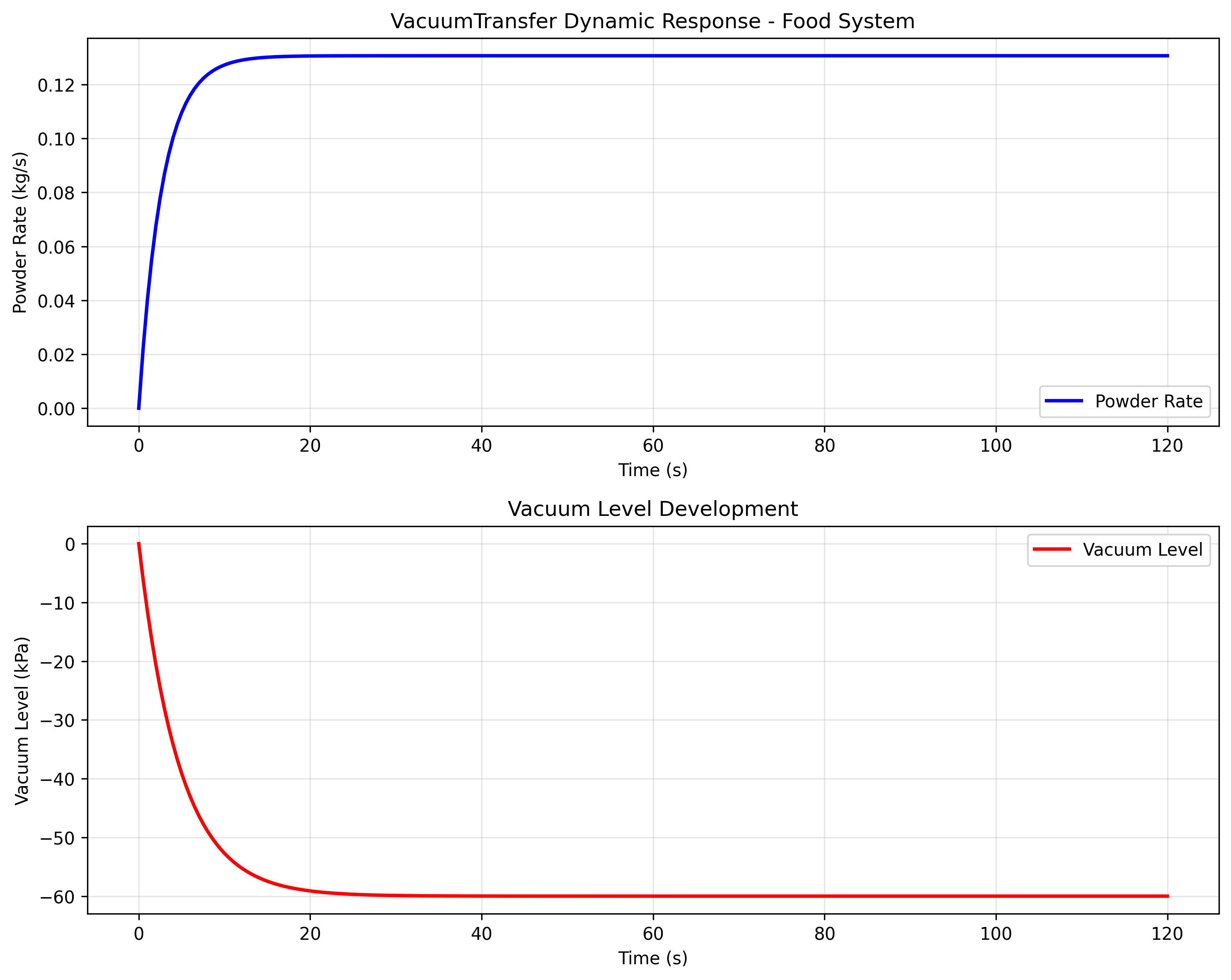
Dynamic response showing powder transfer rate and vacuum level development during system startup.
Detailed Analysis
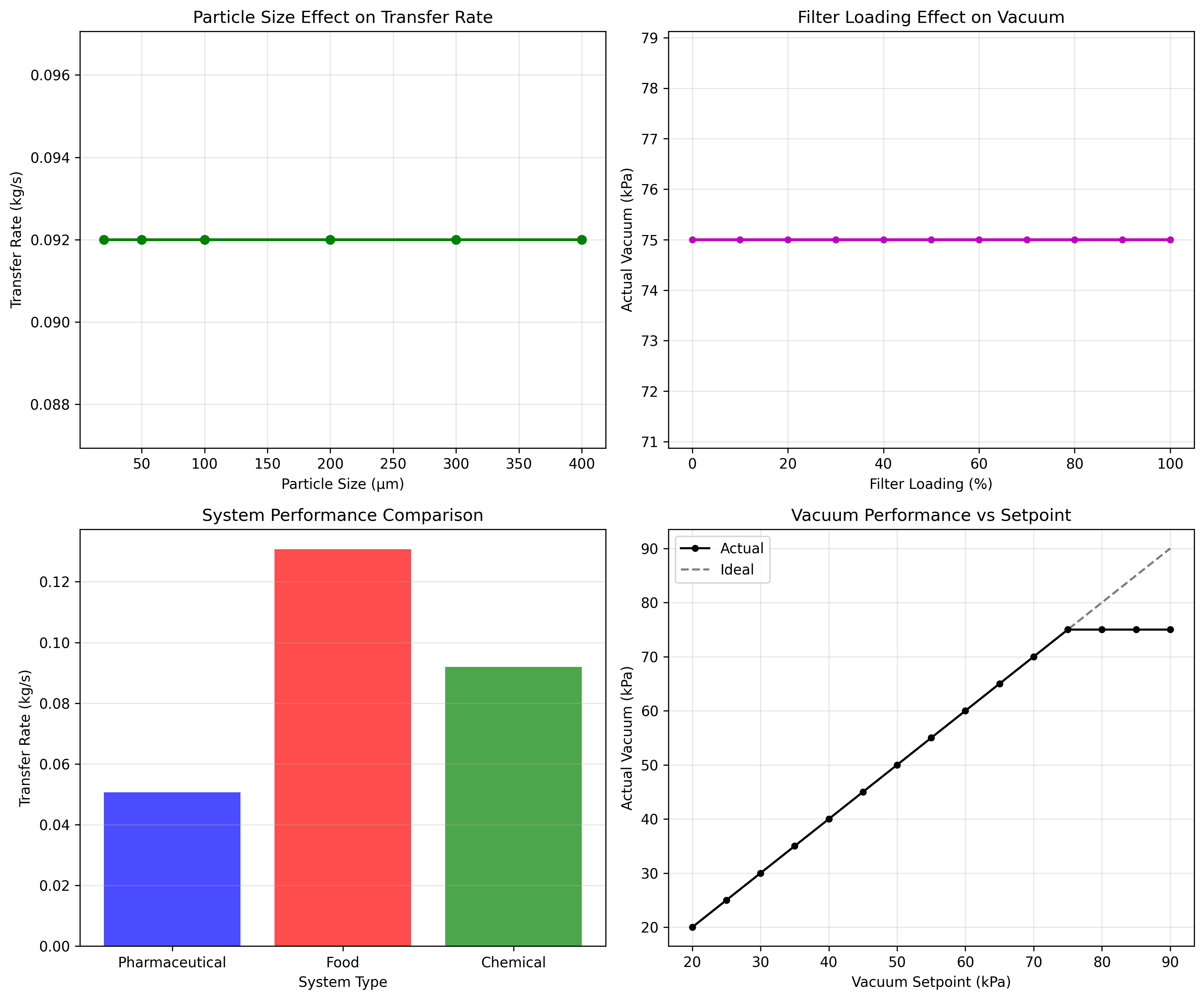
Detailed analysis showing particle size effects, filter loading impacts, system comparisons, and vacuum performance characteristics.
Example Output
=== VacuumTransfer Example ===

1. Creating VacuumTransfer instances:
--------------------------------------
Pharmaceutical vacuum: PharmaVacuumTransfer
  Pump capacity: 80.0 m³/h
  Particle size: 50 μm

Food vacuum: FoodVacuumTransfer
  Pump capacity: 200.0 m³/h
  Particle size: 150 μm

Chemical vacuum: ChemicalVacuumTransfer
  Pump capacity: 150.0 m³/h
  Particle size: 100 μm

2. Steady-state analysis:
-------------------------
Pharmaceutical vacuum results:
  High source, low vacuum:
    Powder rate: 0.05 kg/s
    Vacuum level: -30.0 kPa

  Medium source, medium vacuum:
    Powder rate: 0.05 kg/s
    Vacuum level: -50.0 kPa

  Low source, high vacuum:
    Powder rate: 0.05 kg/s
    Vacuum level: -70.0 kPa

  Full source, max vacuum:
    Powder rate: 0.05 kg/s
    Vacuum level: -75.0 kPa

3. Dynamic simulation:
--------------------
Simulating vacuum system startup with food_vacuum:
Initial conditions: rate=0 kg/s, vacuum=0 Pa
Setpoint: -60 kPa, powder level: 70%

Dynamic simulation results:
  Final powder rate: 0.13 kg/s
  Final vacuum level: -60.0 kPa
  Steady-state time: ~8 s

4. Particle size sensitivity analysis:
--------------------------------------
Chemical vacuum particle size sensitivity (60% powder, -70 kPa):
  20 μm: 0.09 kg/s
  50 μm: 0.09 kg/s
  100 μm: 0.09 kg/s
  200 μm: 0.09 kg/s
  300 μm: 0.09 kg/s
  400 μm: 0.09 kg/s

5. Filter loading effects:
------------------------
Pharma vacuum filter loading effects (80% powder, -80 kPa setpoint):
  0.0 loading: 75.0 kPa actual
  0.1 loading: 75.0 kPa actual
  0.2 loading: 75.0 kPa actual
  0.3 loading: 75.0 kPa actual
  0.4 loading: 75.0 kPa actual
  0.5 loading: 75.0 kPa actual
  0.6 loading: 75.0 kPa actual
  0.7 loading: 75.0 kPa actual
  0.8 loading: 75.0 kPa actual
  0.9 loading: 75.0 kPa actual
  1.0 loading: 75.0 kPa actual

6. Model introspection:
--------------------
Model type: Vacuum Powder Transfer
Description: Pneumatic powder transfer using vacuum pump and cyclone separator

Key parameters:
  vacuum_pump_capacity: 80.0 m³/h - Vacuum pump volumetric capacity
  transfer_line_diameter: 0.04 m - Transfer line internal diameter
  transfer_line_length: 12.0 m - Transfer line length
  powder_density: 500.0 kg/m³ - Powder bulk density
  particle_size: 5e-05 m - Average particle diameter

Key equations:
  air_velocity: v = sqrt(2*ΔP/ρ_air)
  pickup_velocity: v_pickup = 2*sqrt(4*g*d_p*ρ_p/(3*C_d*ρ_air))
  powder_rate: rate = Q_air * ρ_air * loading_ratio * η_cyclone
  pressure_drop: ΔP = Q * (R_line + R_filter)

7. Comparative analysis:
-----------------------
System comparison (70% powder, -60 kPa, 30% filter loading):
  Pharmaceutical : 0.051 kg/s, -60.0 kPa
  Food           : 0.131 kg/s, -60.0 kPa
  Chemical       : 0.092 kg/s, -60.0 kPa

8. Creating visualization plots...
Plots saved as VacuumTransfer_example_plots.png and VacuumTransfer_detailed_analysis.png

=== Example completed successfully ===
Operating Ranges
Material Properties
Bulk Density: 200-1500 kg/m³ (typical powder range)
Particle Size: 10-500 μm (fine to coarse powders)
Powder Level: 0.0-1.0 (source container fill level)
Process Conditions
Vacuum Level: 0 to -100 kPa gauge (typical vacuum range)
Air Velocity: 15-30 m/s (dilute phase transport)
Solids Loading: 0.1-2.0 kg solid/kg air (dilute phase)
Equipment Parameters
Pump Capacity: 10-500 m³/h (laboratory to industrial scale)
Line Diameter: 20-150 mm (typical pneumatic conveying)
Line Length: 1-100 m (practical transfer distances)
Cyclone Efficiency: 80-99% (depends on particle size)
Performance Limits
Filter Loading: 0.0-1.0 (clean to loaded filter)
Transfer Rate: 0.1-50 kg/s (depends on system size)
Response Time: 3-10 s (typical pneumatic system dynamics)
Literature References
Mills, D. (2004). “Pneumatic Conveying Design Guide”, 2nd Edition, Butterworth-Heinemann, ISBN: 978-0750654715.
Klinzing, G.E., Rizk, F., Marcus, R., Leung, L.S. (2010). “Pneumatic Conveying of Solids: A Theoretical and Practical Approach”, 3rd Edition, Springer, ISBN: 978-90-481-3609-4.
Wypych, P.W. (1999). “Handbook of Pneumatic Conveying Engineering”, Marcel Dekker, ISBN: 0-8247-0249-4.
Bradley, D. (1965). “The Hydrocyclone”, Pergamon Press, Oxford.
Muschelknautz, E. (1972). “Design criteria for pneumatic conveying systems”, Bulk Solids Handling, 2(4), 679-684.
Konno, H., Saito, S. (1969). “Pneumatic conveying of solids through straight pipes”, Journal of Chemical Engineering of Japan, 2(2), 211-217.
Weber, M. (1991). “Principles of hydraulic and pneumatic conveying in pipes”, Bulk Solids Handling, 11(1), 57-63.
Gasterstadt, S., Mallick, S.S., Wypych, P.W. (2017). “An investigation into the effect of particle size on dense phase pneumatic conveying”, Particuology, 31, 68-77.