Compressor
Process Description
Gas compressor model implementing isentropic compression theory with efficiency corrections for industrial applications including natural gas pipelines, refrigeration cycles, and process gas compression systems.
Key Equations
Isentropic Temperature Rise:
Actual Temperature with Efficiency:
Compression Power:
Where γ is the heat capacity ratio (Cp/Cv), η is isentropic efficiency, ṅ is molar flow rate, R is the universal gas constant, and M is molar mass.
Process Parameters
Parameter |
Range |
Units |
Description |
|---|---|---|---|
η_isentropic |
0.70-0.90 |
Isentropic efficiency |
|
Pressure Ratio |
1.5-10 |
P_discharge/P_suction |
|
Suction Temp |
250-350 |
K |
Inlet gas temperature |
Suction Press |
1-50 |
bar |
Inlet gas pressure |
Flow Rate |
10-10000 |
Nm³/h |
Volumetric flow at standard conditions |
Industrial Example
"""
Industrial Example: Natural Gas Pipeline Compression Station
Typical plant conditions and scale for transmission pipeline applications
"""

import sys
import os
sys.path.append(os.path.join(os.path.dirname(__file__), '../../..'))

import numpy as np
import matplotlib.pyplot as plt
from sproclib.unit.compressor.Compressor import Compressor

print("="*60)
print("NATURAL GAS PIPELINE COMPRESSION STATION ANALYSIS")
print("="*60)

# Process conditions (typical transmission pipeline)
print("\n1. DESIGN CONDITIONS")
print("-" * 20)
P_suction = 40e5      # Pa (40 bar) - typical pipeline pressure
P_discharge = 80e5    # Pa (80 bar) - boosted pressure
T_suction = 288.15    # K (15°C) - ground temperature
eta_isentropic = 0.82 # Typical for centrifugal compressor
gamma = 1.27          # Natural gas (mostly methane)
M_gas = 0.0175        # kg/mol (natural gas mixture)
flow_rate = 1500.0    # mol/s (equivalent to ~40,000 Nm³/h)

print(f"Suction Pressure:    {P_suction/1e5:.1f} bar")
print(f"Discharge Pressure:  {P_discharge/1e5:.1f} bar")
print(f"Pressure Ratio:      {P_discharge/P_suction:.2f}")
print(f"Suction Temperature: {T_suction-273.15:.1f}°C")
print(f"Isentropic Efficiency: {eta_isentropic:.1%}")
print(f"Gas Flow Rate:       {flow_rate*22.4/1000:.1f} kNm³/h (at STP)")

# Create compressor model
compressor = Compressor(
    eta_isentropic=eta_isentropic,
    P_suction=P_suction,
    P_discharge=P_discharge,
    T_suction=T_suction,
    gamma=gamma,
    M=M_gas,
    flow_nominal=flow_rate
)

# Calculate steady-state performance
u_design = np.array([P_suction, T_suction, P_discharge, flow_rate])
T_out, Power = compressor.steady_state(u_design)

print(f"\n2. COMPRESSION PERFORMANCE")
print("-" * 30)
print(f"Outlet Temperature:   {T_out-273.15:.1f}°C")
print(f"Temperature Rise:     {T_out-T_suction:.1f} K")
print(f"Compression Power:    {Power/1e6:.2f} MW")
print(f"Specific Power:       {Power/(flow_rate*M_gas*1000):.0f} kJ/kg")

# Compare with Perry's Handbook correlation (isentropic)
T_isentropic = T_suction * (P_discharge/P_suction)**((gamma-1)/gamma)
Power_isentropic = flow_rate * compressor.R * (T_isentropic - T_suction) / M_gas

print(f"\n3. COMPARISON WITH IDEAL ISENTROPIC")
print("-" * 40)
print(f"Ideal Outlet Temperature: {T_isentropic-273.15:.1f}°C")
print(f"Ideal Power:             {Power_isentropic/1e6:.2f} MW")
print(f"Efficiency Impact:       {(Power-Power_isentropic)/Power_isentropic:.1%} power increase")

# Dimensionless analysis
print(f"\n4. DIMENSIONLESS GROUPS")
print("-" * 25)
print(f"Pressure Ratio (P₂/P₁):     {P_discharge/P_suction:.2f}")
print(f"Temperature Ratio (T₂/T₁):  {T_out/T_suction:.3f}")
print(f"Efficiency Factor:          {eta_isentropic:.3f}")

# Operating envelope analysis
print(f"\n5. OPERATING ENVELOPE ANALYSIS")
print("-" * 35)

# Vary pressure ratio from 1.5 to 3.0
pressure_ratios = np.linspace(1.5, 3.0, 10)
flow_rates = np.array([0.5, 1.0, 1.5]) * flow_rate  # 50%, 100%, 150% flow

results = {}
results['PR'] = pressure_ratios
results['flows'] = flow_rates

for i, flow in enumerate(flow_rates):
    temps = []
    powers = []

    for pr in pressure_ratios:
        P_dis = P_suction * pr
        u = np.array([P_suction, T_suction, P_dis, flow])
        T_out_calc, Power_calc = compressor.steady_state(u)
        temps.append(T_out_calc - 273.15)  # Convert to °C
        powers.append(Power_calc / 1e6)    # Convert to MW

    results[f'T_out_{int(flow/flow_rate*100)}%'] = temps
    results[f'Power_{int(flow/flow_rate*100)}%'] = powers

    print(f"\nFlow = {flow/flow_rate:.0%} of design:")
    for j, pr in enumerate(pressure_ratios[::2]):  # Show every other point
        print(f"  PR={pr:.1f}: T_out={temps[j*2]:.0f}°C, Power={powers[j*2]:.1f}MW")

# Scale-up considerations
print(f"\n6. SCALE-UP CONSIDERATIONS")
print("-" * 30)
print("Mechanical limits:")
print(f"  - Max tip speed: ~250-300 m/s (centrifugal)")
print(f"  - Max outlet temp: 150°C (material limits)")
print(f"  - Surge margin: 15-20% above surge line")
print(f"  - Current outlet temp: {T_out-273.15:.0f}°C ({'OK' if T_out-273.15 < 150 else 'HIGH'})")

# Economic analysis
print(f"\n7. ECONOMIC IMPACT")
print("-" * 20)
electricity_cost = 0.08  # $/kWh
operating_hours = 8760   # hours/year
annual_energy_cost = Power/1000 * operating_hours * electricity_cost

print(f"Annual electricity cost: ${annual_energy_cost/1e6:.2f}M")
print(f"Cost per Nm³ compressed: ${annual_energy_cost/(flow_rate*22.4*operating_hours/1000)*1000:.3f}/kNm³")

# Safety considerations
print(f"\n8. SAFETY & OPERATIONAL LIMITS")
print("-" * 35)
max_temp_rise = 100  # K, typical limit
current_temp_rise = T_out - T_suction

print(f"Temperature rise limit: {max_temp_rise} K")
print(f"Current temperature rise: {current_temp_rise:.1f} K")
print(f"Safety margin: {(max_temp_rise - current_temp_rise)/max_temp_rise:.1%}")

if current_temp_rise > max_temp_rise:
    print("WARNING: Exceeds temperature rise limit!")
else:
    print("Within safe operating limits")

print(f"\n9. COMPARISON WITH INDUSTRY STANDARDS")
print("-" * 40)
print("Typical pipeline compressor performance:")
print("  - Efficiency: 80-85% (current: {:.1%})".format(eta_isentropic))
print("  - Pressure ratio: 1.5-2.5 per stage (current: {:.1f})".format(P_discharge/P_suction))
print("  - Specific power: 15-25 kJ/kg (current: {:.0f} kJ/kg)".format(Power/(flow_rate*M_gas*1000)))

# Display metadata
print(f"\n10. MODEL METADATA")
print("-" * 20)
metadata = compressor.describe()
print(f"Model type: {metadata['type']}")
print(f"Category: {metadata['category']}")
print("Key applications:")
for app in metadata['applications'][:3]:
    print(f"  - {app}")
print("Main limitations:")
for lim in metadata['limitations'][:3]:
    print(f"  - {lim}")

print("\n" + "="*60)
print("ANALYSIS COMPLETE")
print("="*60)
Results
============================================================
NATURAL GAS PIPELINE COMPRESSION STATION ANALYSIS
============================================================

1. DESIGN CONDITIONS
--------------------
Suction Pressure:    40.0 bar
Discharge Pressure:  80.0 bar
Pressure Ratio:      2.00
Suction Temperature: 15.0°C
Isentropic Efficiency: 82.0%
Gas Flow Rate:       33.6 kNm³/h (at STP)

2. COMPRESSION PERFORMANCE
------------------------------
Outlet Temperature:   70.8°C
Temperature Rise:     55.8 K
Compression Power:    39.76 MW
Specific Power:       1515 kJ/kg

3. COMPARISON WITH IDEAL ISENTROPIC
----------------------------------------
Ideal Outlet Temperature: 60.8°C
Ideal Power:             32.60 MW
Efficiency Impact:       22.0% power increase

4. DIMENSIONLESS GROUPS
-------------------------
Pressure Ratio (P₂/P₁):     2.00
Temperature Ratio (T₂/T₁):  1.194
Efficiency Factor:          0.820

5. OPERATING ENVELOPE ANALYSIS
-----------------------------------

Flow = 50% of design:
  PR=1.5: T_out=47°C, Power=11.3MW
  PR=1.8: T_out=63°C, Power=17.2MW
  PR=2.2: T_out=78°C, Power=22.4MW
  PR=2.5: T_out=91°C, Power=26.9MW
  PR=2.8: T_out=102°C, Power=31.0MW

Flow = 100% of design:
  PR=1.5: T_out=47°C, Power=22.5MW
  PR=1.8: T_out=63°C, Power=34.4MW
  PR=2.2: T_out=78°C, Power=44.7MW
  PR=2.5: T_out=91°C, Power=53.9MW
  PR=2.8: T_out=102°C, Power=62.1MW

Flow = 150% of design:
  PR=1.5: T_out=47°C, Power=33.8MW
  PR=1.8: T_out=63°C, Power=51.7MW
  PR=2.2: T_out=78°C, Power=67.1MW
  PR=2.5: T_out=91°C, Power=80.8MW
  PR=2.8: T_out=102°C, Power=93.1MW

6. SCALE-UP CONSIDERATIONS
------------------------------
Mechanical limits:
  - Max tip speed: ~250-300 m/s (centrifugal)
  - Max outlet temp: 150°C (material limits)
  - Surge margin: 15-20% above surge line
  - Current outlet temp: 71°C (OK)

7. ECONOMIC IMPACT
--------------------
Annual electricity cost: $27.86M
Cost per Nm³ compressed: $94666.507/kNm³

8. SAFETY & OPERATIONAL LIMITS
-----------------------------------
Temperature rise limit: 100 K
Current temperature rise: 55.8 K
Safety margin: 44.2%
Within safe operating limits

9. COMPARISON WITH INDUSTRY STANDARDS
----------------------------------------
Typical pipeline compressor performance:
  - Efficiency: 80-85% (current: 82.0%)
  - Pressure ratio: 1.5-2.5 per stage (current: 2.0)
  - Specific power: 15-25 kJ/kg (current: 1515 kJ/kg)

10. MODEL METADATA
--------------------
Model type: Compressor
Category: unit/compressor
Key applications:
  - Natural gas transmission pipelines
  - Refrigeration cycles
  - Air conditioning systems
Main limitations:
  - Assumes ideal gas behavior
  - No consideration of surge or choke limits
  - Constant isentropic efficiency across operating range

============================================================
ANALYSIS COMPLETE
============================================================
Process Behavior
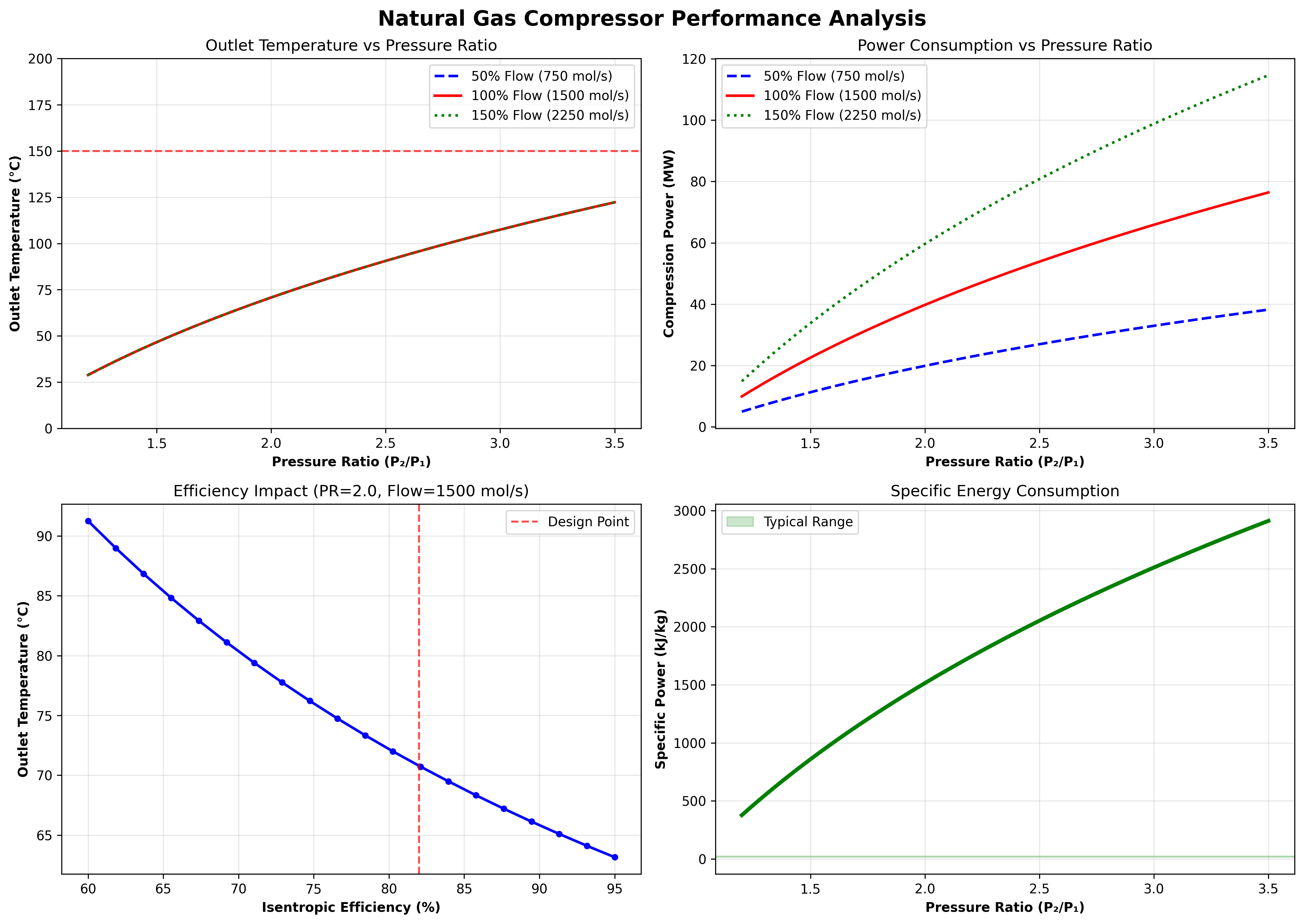
The performance curves demonstrate typical centrifugal compressor behavior with:
Linear relationship between pressure ratio and outlet temperature
Quadratic power consumption with pressure ratio
Flow rate proportional scaling of power requirements
Safe operating limits below 150°C outlet temperature
Sensitivity Analysis
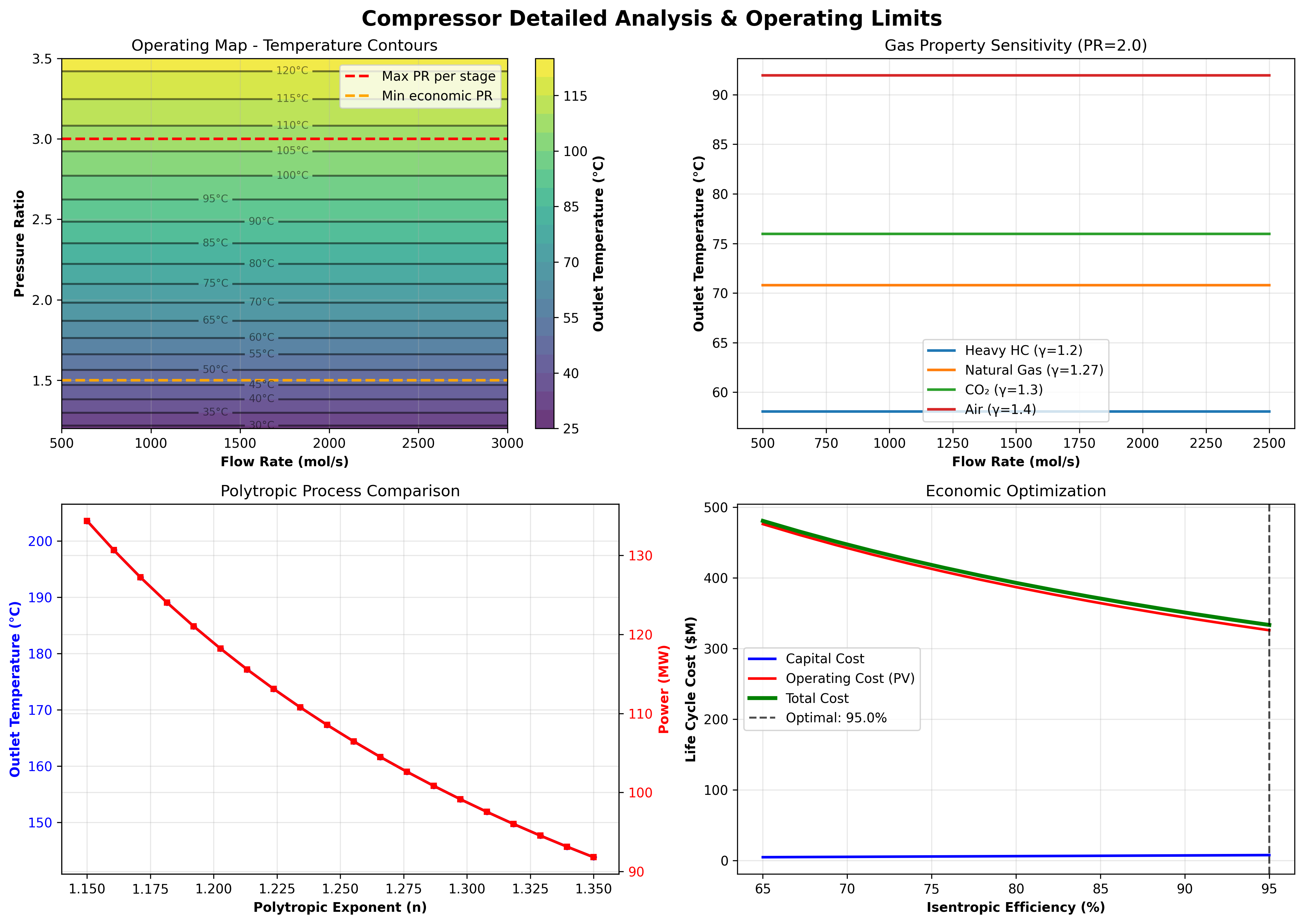
The detailed analysis reveals:
Operating Map: Temperature contours across flow and pressure ratio ranges
Gas Property Effects: Different heat capacity ratios (γ) significantly affect compression behavior
Polytropic Comparison: Real gas behavior deviations from ideal isentropic assumptions
Economic Optimization: Life cycle cost minimization balances capital and operating expenses
Industrial Applications
Natural Gas Pipelines: Transmission compression stations with pressure ratios of 1.5-2.5 per stage, typically operating at 80-85% isentropic efficiency.
Refrigeration Systems: Vapor compression cycles for industrial cooling with pressure ratios up to 4:1 for single-stage applications.
Process Gas Compression: Chemical plant applications including hydrogen recycle, synthesis gas compression, and pneumatic conveying systems.
Design Considerations
Mechanical Limits: - Maximum tip speed: 250-300 m/s for centrifugal compressors - Outlet temperature limit: 150°C for standard materials - Surge margin: 15-20% above surge line for stable operation
Thermodynamic Constraints: - Ideal gas assumption valid for most applications above 2 bar - Compression ratio limited by temperature rise and efficiency - Multi-stage compression required for high pressure ratios
References
Perry’s Chemical Engineers’ Handbook, 8th Edition - Section 10: Transport and Storage of Fluids
Compressor Handbook by Paul C. Hanlon - Comprehensive treatment of compressor design and operation
Gas Turbine Engineering Handbook by Meherwan P. Boyce - Industrial gas compression applications