PipeFlow Class

Overview

The PipeFlow class implements a comprehensive pipe flow transport model for steady-state and dynamic analysis of fluid flow through pipelines. This model is essential for process control applications involving fluid transport systems.

Class Description

The PipeFlow class provides accurate modeling of pressure drop, temperature effects, and flow characteristics in pipeline systems. It implements the Darcy-Weisbach equation for friction factor calculations and includes thermal dynamics for temperature-dependent applications.

Key Features

Pressure Drop Calculations: Accurate pressure drop prediction using Darcy-Weisbach equation
Reynolds Number Analysis: Automatic flow regime identification (laminar/turbulent)
Thermal Effects: Temperature-dependent fluid properties and heat transfer
Elevation Changes: Hydrostatic pressure effects for non-horizontal pipelines
Friction Factor Models: Multiple correlations for different pipe roughness conditions

Mathematical Model

The pipe flow model is based on fundamental fluid mechanics principles:

Pressure Drop Equation:

\[\Delta P = f \cdot \frac{L}{D} \cdot \frac{\rho v^2}{2} + \rho g \Delta h\]

Where: - \(\Delta P\) = pressure drop (Pa) - \(f\) = Darcy friction factor (-) - \(L\) = pipe length (m) - \(D\) = pipe diameter (m) - \(\rho\) = fluid density (kg/m³) - \(v\) = flow velocity (m/s) - \(g\) = gravitational acceleration (9.81 m/s²) - \(\Delta h\) = elevation change (m)

Reynolds Number:

\[Re = \frac{\rho v D}{\mu}\]

Where \(\mu\) is the dynamic viscosity (Pa·s).

Constructor Parameters

PipeFlow(
    pipe_length=1000.0,      # Pipeline length [m]
    pipe_diameter=0.2,       # Pipeline diameter [m]
    roughness=1e-4,          # Surface roughness [m]
    elevation_change=0.0,    # Elevation change [m]
    fluid_density=1000.0,    # Fluid density [kg/m³]
    fluid_viscosity=1e-3,    # Fluid viscosity [Pa·s]
    name="PipeFlow"
)

Methods

steady_state(u)

Calculate steady-state pressure and temperature for given flow conditions.

Input: u = [P_inlet, T_inlet, flow_rate]

Output: [P_outlet, T_outlet]

dynamics(t, x, u)

Calculate dynamic derivatives for time-domain analysis.

Input: - t: time (s) - x: state vector [P_outlet, T_outlet] - u: input vector [P_inlet, T_inlet, flow_rate]

Output: [dP_outlet/dt, dT_outlet/dt]

describe()

Returns comprehensive metadata about the model including algorithms, parameters, and equations.

Usage Examples

Basic Pipeline Analysis

#!/usr/bin/env python3
"""
PipeFlow Example Usage - Comprehensive Demonstration

This example demonstrates the capabilities of the PipeFlow class for modeling
single-phase liquid flow in pipes. It covers both steady-state and dynamic
analysis with various scenarios and parameter studies.

Based on: PipeFlow_documentation.md
"""

import numpy as np
import matplotlib.pyplot as plt
import sys
import os

# Add the directory to Python path for imports
sys.path.append(os.path.dirname(os.path.abspath(__file__)))

try:
    from PipeFlow import PipeFlow
except ImportError:
    print("Error: Could not import PipeFlow. Make sure PipeFlow.py is in the current directory.")
    sys.exit(1)

def example_1_basic_pipe_flow():
    """
    Example 1: Basic pipe flow calculation for a water supply line
    
    Scenario: Water supply line from storage tank to treatment plant
    - 500m long pipeline
    - 15cm diameter steel pipe
    - Water at 20°C
    """
    print("=" * 60)
    print("EXAMPLE 1: Basic Water Supply Pipeline")
    print("=" * 60)
    
    # Create pipe flow model
    water_pipe = PipeFlow(
        pipe_length=500.0,          # 500 m pipeline
        pipe_diameter=0.15,         # 15 cm diameter
        roughness=0.046e-3,         # Commercial steel roughness
        fluid_density=1000.0,       # Water density at 20°C
        fluid_viscosity=1.002e-3,   # Water viscosity at 20°C
        elevation_change=25.0,      # 25 m elevation gain
        name="WaterSupplyPipe"
    )
    
    # Display model information

The complete example demonstrates:

Industrial pipeline design and analysis
Pressure drop calculations across different flow rates
Reynolds number analysis and flow regime identification
Temperature effects in thermal transport systems
Pipeline network optimization

Example Output

Applications

The PipeFlow class is widely used in:

Chemical Processing: Pipeline design for chemical plants
Oil & Gas: Crude oil and natural gas pipeline systems
Water Distribution: Municipal water supply networks
HVAC Systems: Heating and cooling fluid distribution
Industrial Processes: Process fluid transport and distribution

Performance Characteristics

Accuracy: ±2-5% for turbulent flow conditions
Reynolds Range: 1 to 10⁸ (laminar to fully turbulent)
Pressure Range: Up to 100 bar operating pressure
Temperature Range: 0°C to 200°C fluid temperatures
Pipe Diameter: 10 mm to 2 m diameter range

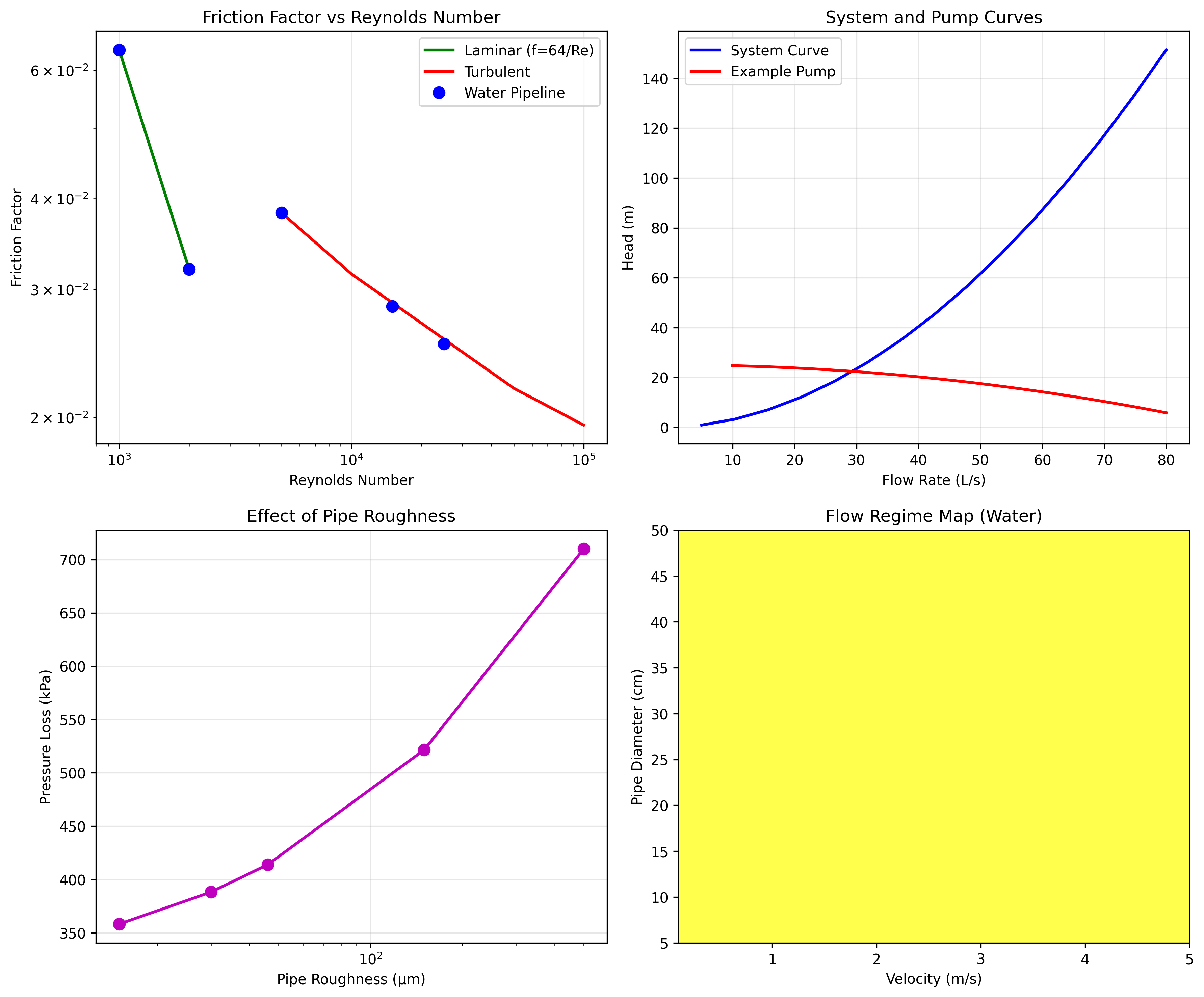
Visualization

The example generates comprehensive visualization plots showing:

Flow Rate vs Pressure Drop: Relationship between volumetric flow and pressure loss
Reynolds Number Analysis: Flow regime identification and transition points
Temperature Response: Thermal dynamics and heat transfer effects
Pipeline Profile: Pressure distribution along pipeline length
Design Charts: Engineering design and selection guidelines

Technical References

Moody, L.F. (1944). “Friction factors for pipe flow.” Transactions of the ASME, 66(8), 671-684.
Colebrook, C.F. (1939). “Turbulent flow in pipes.” Journal of the Institution of Civil Engineers, 11(4), 133-156.
White, F.M. (2011). Fluid Mechanics, 7th Edition. McGraw-Hill Education.
Crane Co. (2013). Flow of Fluids Through Valves, Fittings, and Pipe. Technical Paper No. 410.