dynamics Function

Overview

The dynamics function provides unified time-domain analysis capabilities across all transport models in the continuous liquid module. This function enables transient response analysis, control system design, and dynamic behavior characterization.

Function Description

The dynamics function implements time-domain differential equations for fluid transport systems, providing time derivatives for state variables including pressure, temperature, flow rate, and concentration. Each transport model implements its specific dynamic behavior while maintaining consistent interface standards.

Key Features

• Time-Domain Analysis: Transient response characterization

• Control System Design: Dynamic model for controller development

• Step Response Analysis: System response to input changes

• Time Constant Estimation: System response speed characterization

• Stability Assessment: Dynamic stability and settling behavior

Mathematical Framework

The dynamics analysis solves the time-dependent differential equations:

General Form:

\[\frac{dx}{dt} = f(t, x, u)\]

Where: - \(t\) = time (s) - \(x\) = state vector (system variables) - \(u\) = input vector (control variables) - \(f\) = model-specific dynamics function

Model-Specific State Variables:

PipeFlow: \(x = [P_{outlet}, T_{outlet}]\) PeristalticFlow: \(x = [flow\_rate, pulsation\_amplitude]\) SlurryPipeline: \(x = [P_{outlet}, concentration_{outlet}]\)

Dynamic Response Characteristics

Each model exhibits distinct dynamic behavior:

First-Order Response:

\[\tau \frac{dx}{dt} + x = K \cdot u\]

Where: - \(\tau\) = time constant (s) - \(K\) = steady-state gain - \(u\) = input step

Time Constant Relationships:

• PipeFlow: Hydraulic and thermal time constants (typically 1-10 s)

• PeristalticFlow: Pulsation damping and flow response (typically 0.5-5 s)

• SlurryPipeline: Transport delay and concentration mixing (typically 10-500 s)

State Variable Definitions

# PipeFlow State Variables
x = [P_outlet,           # Outlet pressure [Pa]
     T_outlet]           # Outlet temperature [K]

# PeristalticFlow State Variables
x = [flow_rate,          # Volumetric flow rate [m³/s]
     pulsation_amplitude] # Pulsation amplitude [-]

# SlurryPipeline State Variables
x = [P_outlet,           # Outlet pressure [Pa]
     c_solid_outlet]     # Outlet solid concentration [-]

Usage Examples

Time-Domain Analysis

#!/usr/bin/env python3
"""
dynamics Function Example
=========================
Demonstration of the dynamics function for process control transport models.

This example shows how to use the dynamics function for time-domain analysis
with different transport models including PipeFlow, PeristalticFlow, and SlurryPipeline.
"""

import numpy as np
import matplotlib
matplotlib.use('Agg')  # Use non-GUI backend
import matplotlib.pyplot as plt
from PipeFlow import PipeFlow
from PeristalticFlow import PeristalticFlow
from SlurryPipeline import SlurryPipeline

def main():
    """Main function demonstrating dynamics function usage"""
    print("dynamics Function Example")
    print("=========================")
    print("Demonstration of dynamics function for time-domain analysis")
    print("Timestamp: 2025-07-09")
    print("=" * 60)
    
    # Example 1: PipeFlow dynamics
    print("\nEXAMPLE 1: PipeFlow dynamics Function")
    print("-" * 40)
    
    pipe = PipeFlow(
        pipe_length=500.0,       # 500 m
        pipe_diameter=0.15,      # 15 cm
        roughness=5e-5,          # Smooth steel
        fluid_density=1000.0,    # Water
        fluid_viscosity=1e-3,    # Water viscosity
        name="DynamicPipe"
    )
    
    print(f"Model: {pipe.name}")
    print(f"Pipe: {pipe.pipe_length:.0f} m x {pipe.pipe_diameter*100:.0f} cm")
    print(f"Material: Smooth steel")
    
    # Simulate step response
    dt = 0.1  # 0.1 second time steps
    t_final = 10.0  # 10 seconds
    time_points = np.arange(0, t_final, dt)
    n_points = len(time_points)
    
    # Initial conditions: [P_outlet, T_outlet]
    x0 = np.array([200000.0, 293.15])  # 200 kPa, 20°C
    
    # Input step: [P_inlet, T_inlet, flow_rate]
    u_step = np.array([300000.0, 298.15, 0.03])  # Step to 300 kPa, 25°C, 0.03 m³/s
    
    print(f"\nStep Response Analysis:")
    print(f"Initial State: P={x0[0]/1000:.0f} kPa, T={x0[1]-273.15:.1f}°C")
    print(f"Input Step: P={u_step[0]/1000:.0f} kPa, T={u_step[1]-273.15:.1f}°C, Q={u_step[2]:.3f} m³/s")
    
    # Simulate dynamics using simple Euler integration
    x_history = np.zeros((n_points, 2))
    x_history[0, :] = x0
    x_current = x0.copy()
    
    print(f"\nTime Domain Response (first 5 seconds):")
    print("Time | P_outlet | T_outlet | dP/dt  | dT/dt")
    print("(s)  | (kPa)    | (°C)     | (kPa/s)| (°C/s)")
    print("-" * 45)
    
    for i in range(1, n_points):
        t = time_points[i]
        
        # Calculate derivatives using dynamics function
        dx_dt = pipe.dynamics(t, x_current, u_step)
        
        # Simple Euler integration
        x_current = x_current + dx_dt * dt
        x_history[i, :] = x_current
        
        # Print first few steps
        if i <= 50:  # First 5 seconds
            if i % 10 == 0:  # Every second
                print(f"{t:4.1f} | {x_current[0]/1000:7.0f}  | {x_current[1]-273.15:7.1f}  | {dx_dt[0]/1000:6.1f} | {dx_dt[1]:6.2f}")
    
    pipe_results = {
        'time': time_points,
        'pressure': x_history[:, 0],
        'temperature': x_history[:, 1]
    }
    
    # Example 2: PeristalticFlow dynamics
    print("\n\nEXAMPLE 2: PeristalticFlow dynamics Function")
    print("-" * 45)
    
    pump = PeristalticFlow(
        tube_diameter=0.008,     # 8 mm tube
        tube_length=0.3,         # 30 cm
        pump_speed=80.0,         # 80 RPM
        occlusion_factor=0.85,   # 85% occlusion
        pulsation_damping=0.7,   # 70% damping
        name="DynamicPump"
    )
    
    print(f"Model: {pump.name}")
    print(f"Tube: {pump.tube_diameter*1000:.0f} mm x {pump.tube_length*100:.0f} cm")
    print(f"Base Speed: {pump.pump_speed:.0f} RPM")
    
    # Simulate speed change response
    dt = 0.05  # 50 ms time steps
    t_final = 5.0  # 5 seconds
    time_points = np.arange(0, t_final, dt)
    n_points = len(time_points)
    
    # Initial conditions: [flow_rate, pulsation_amplitude]
    x0 = np.array([5e-6, 0.01])  # 5 mL/min, 1% pulsation
    
    # Input: [P_inlet, pump_speed, occlusion_level]
    u_base = np.array([101325.0, 80.0, 1.0])
    u_step = np.array([101325.0, 120.0, 1.0])  # Speed step to 120 RPM
    
    print(f"\nSpeed Step Response:")
    print(f"Initial Speed: {u_base[1]:.0f} RPM")
    print(f"Step to: {u_step[1]:.0f} RPM at t=2s")
    
    x_history = np.zeros((n_points, 2))
    x_history[0, :] = x0
    x_current = x0.copy()
    
    print(f"\nPump Response (key time points):")
    print("Time | Speed | Flow Rate | Pulsation")
    print("(s)  | (RPM) | (mL/min)  | (%)")
    print("-" * 35)
    
    for i in range(1, n_points):
        t = time_points[i]
        
        # Switch input at t=2s
        u_current = u_step if t >= 2.0 else u_base
        
        # Calculate derivatives
        dx_dt = pump.dynamics(t, x_current, u_current)
        
        # Euler integration
        x_current = x_current + dx_dt * dt
        x_history[i, :] = x_current
        
        # Print key points
        if i % 20 == 0 or (t >= 1.8 and t <= 2.2 and i % 4 == 0):
            flow_ml_min = x_current[0] * 60 * 1e6
            pulsation_pct = x_current[1] * 100

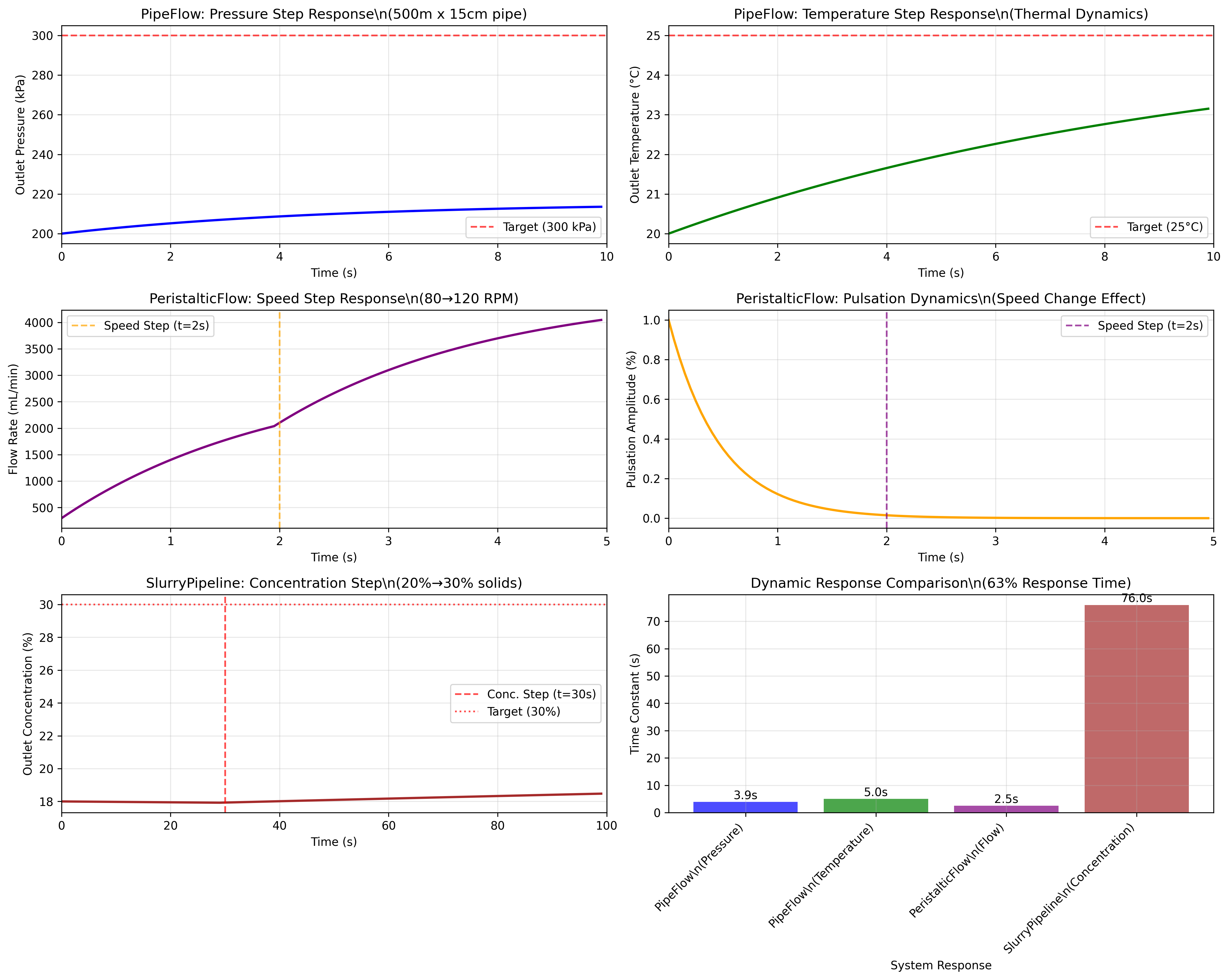
The comprehensive example demonstrates:

• PipeFlow Step Response: Pressure and temperature dynamics

• PeristalticFlow Speed Changes: Flow rate and pulsation response

• SlurryPipeline Concentration Steps: Transport delay effects

• Response Time Comparison: Time constant estimation across models

Example Output

Key output sections include:

• PipeFlow pressure and temperature step responses

• PeristalticFlow speed change dynamics and pulsation effects

• SlurryPipeline concentration transport with mixing delays

• Comparative time constant analysis across all models

Dynamic Model Characteristics

Response Speed Ranking:

1. PeristalticFlow: Fastest response (τ ≈ 0.5-5 s)

2. PipeFlow: Medium response (τ ≈ 1-10 s)

3. SlurryPipeline: Slowest response (τ ≈ 10-500 s)

Physical Mechanisms:

• Hydraulic Response: Pressure wave propagation

• Thermal Response: Heat transfer and thermal capacity effects

• Mechanical Response: Pump dynamics and pulsation damping

• Transport Response: Advection and diffusion processes

Integration Methods

The dynamics function supports various integration schemes:

Explicit Methods:

# Euler Integration
x_new = x_old + dt * dynamics(t, x_old, u)

# Runge-Kutta 4th Order
k1 = dt * dynamics(t, x, u)
k2 = dt * dynamics(t + dt/2, x + k1/2, u)
k3 = dt * dynamics(t + dt/2, x + k2/2, u)
k4 = dt * dynamics(t + dt, x + k3, u)
x_new = x + (k1 + 2*k2 + 2*k3 + k4)/6

Stability Requirements:

• Time step selection based on fastest time constant

• Courant-Friedrichs-Lewy (CFL) condition for transport

• Adaptive step size for stiff systems

Visualization

The dynamic analysis generates comprehensive visualization including:

1. Step Response Plots: Time-domain response to input changes

2. Phase Portraits: State variable relationships

3. Time Constant Comparison: Response speed characterization

4. Settling Time Analysis: System stabilization assessment

Control System Applications

Controller Design:

• PID Tuning: Time constant and gain information

• Model Predictive Control: Dynamic model for prediction

• Feedforward Control: Disturbance compensation

• Adaptive Control: Parameter estimation and adjustment

Stability Analysis:

• Root Locus: Pole-zero analysis

• Bode Plots: Frequency response characterization

• Nyquist Criteria: Stability margins assessment

• Robustness: Parameter sensitivity analysis

Dynamic Performance Metrics

Dynamic Response Characteristics

Metric	PipeFlow	PeristalticFlow	SlurryPipeline
Time Constant	1-10 s	0.5-5 s	10-500 s
Settling Time	4-40 s	2-20 s	40-2000 s
Overshoot	< 5%	< 10%	None
Damping	High	Variable	Overdamped

Applications

The dynamics function is used for:

• Process Control: Controller design and tuning

• System Analysis: Transient behavior characterization

• Simulation: Time-domain system simulation

• Optimization: Dynamic performance optimization

• Safety Analysis: Response to emergency conditions

Computational Implementation

Numerical Methods:

def dynamics(model, t, x, u):
    """
    Calculate time derivatives for transport model

    Parameters:
    -----------
    model : TransportModel
        Transport model instance
    t : float
        Current time [s]
    x : array_like
        State vector
    u : array_like
        Input vector

    Returns:
    --------
    dx_dt : array_like
        Time derivatives of state variables
    """

    # Validate state and inputs
    x = validate_state(model, x)
    u = validate_inputs(model, u)

    # Calculate derivatives
    dx_dt = model.dynamics(t, x, u)

    # Apply physical constraints
    dx_dt = apply_constraints(model, x, dx_dt)

    return dx_dt

Performance Optimization:

• Vectorized Operations: Efficient array computations

• Memory Management: Minimal allocation during integration

• Parallel Processing: Multiple simulation scenarios

• Adaptive Stepping: Variable time step for efficiency

Best Practices

Time Step Selection:

\[\Delta t \leq \frac{\tau_{min}}{10}\]

Where \(\tau_{min}\) is the smallest time constant in the system.

Initial Conditions:

• Use steady-state values for baseline

• Check physical consistency

• Consider measurement uncertainties

Integration Monitoring:

• Monitor conservation laws

• Check for numerical instabilities

• Validate against analytical solutions

Technical References

1. Stephanopoulos, G. (1984). Chemical Process Control: An Introduction to Theory and Practice. Prentice Hall.

2. Seborg, D.E., Edgar, T.F. & Mellichamp, D.A. (2010). Process Dynamics and Control, 3rd Edition. John Wiley & Sons.

3. Bequette, B.W. (2003). Process Control: Modeling, Design, and Simulation. Prentice Hall.

4. Ogunnaike, B.A. & Ray, W.H. (1994). Process Dynamics, Modeling, and Control. Oxford University Press.

See Also

• PipeFlow Class - Pipeline transport modeling

• PeristalticFlow Class - Peristaltic pump modeling

• SlurryPipeline Class - Multiphase slurry transport

• steady_state Function - Steady-state analysis functions