Plug Flow Reactor (PFR)

Overview

The Plug Flow Reactor (PFR) model simulates tubular reactors with axial discretization where fluid elements move through the reactor as “plugs” without back-mixing. It is widely used for gas-phase reactions, high-temperature processes, and situations where high conversion and precise residence time control are required.

Theory and Equations

Material Balance (per segment)

\[\frac{dC_A}{dt} = -u \frac{dC_A}{dz} - k(T) C_A\]

Energy Balance (per segment)

\[\frac{dT}{dt} = -u \frac{dT}{dz} + \frac{(-\Delta H_r) k(T) C_A}{\rho c_p} + \frac{UA(T_w - T)}{\rho c_p V_{seg}}\]

where: - \(u\) = superficial velocity [m/s] - \(z\) = axial position [m] - \(T_w\) = wall temperature [K] - \(V_{seg}\) = segment volume [m³]

Reaction Kinetics

\[k(T) = k_0 \exp\left(\frac{-E_a}{RT}\right)\]

Axial Discretization

The reactor is divided into n_segments: - Segment length: \(\Delta z = L / n_{segments}\) - Segment volume: \(V_{seg} = A_{cross} \times \Delta z\)

Parameters

Design Parameters

• L: Reactor length [m] (1-100 m)

• A_cross: Cross-sectional area [m²] (0.01-10 m²)

• D_tube: Tube diameter [m] (0.05-2.0 m)

• n_segments: Number of discretization segments (10-200)

Usage Example

Basic Implementation

from unit.reactor.PlugFlowReactor import PlugFlowReactor
import numpy as np

# Create PFR instance
reactor = PlugFlowReactor(
    L=10.0,                # Reactor length [m]
    A_cross=0.1,           # Cross-sectional area [m²]
    n_segments=20,         # Number of segments
    k0=1e8,                # Pre-exponential factor [1/min]
    Ea=60000.0             # Activation energy [J/mol]
)

# Operating conditions
u = np.array([50.0, 2.0, 400.0, 380.0])  # [q, CAi, Ti, Tw]

# Calculate steady-state profiles
x_ss = reactor.steady_state(u)
conversion = reactor.calculate_conversion(x_ss)

Example Output

Running the complete example produces:

============================================================
PlugFlowReactor (PFR) Example
============================================================
Reactor: Example_PFR
Length: 10.0 m
Cross-sectional area: 0.1 m²
Number of segments: 20
Segment length: 0.500 m

Steady-State Analysis:
------------------------------
Overall conversion: 2.7%
Inlet concentration: 1.997 mol/L
Outlet concentration: 1.942 mol/L
Residence time: 0.02 min
Superficial velocity: 0.0083 m/s

Parametric Study - Flow Rate Effect:
----------------------------------------
Flow rate:   10.0 L/min → Conversion: 13.0%
Flow rate:   50.0 L/min → Conversion: 2.7%
Flow rate:  200.0 L/min → Conversion: 0.7%

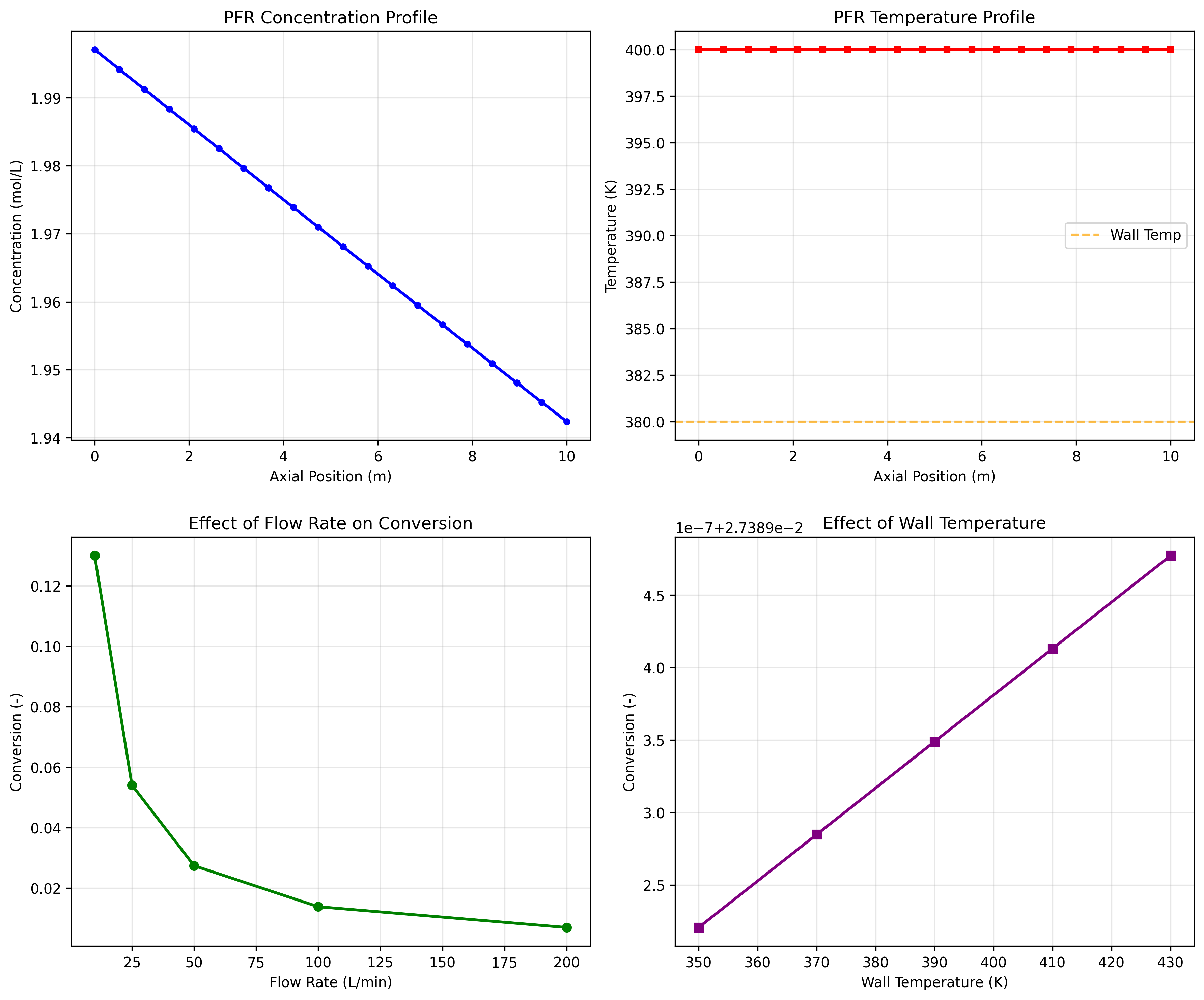
Performance Plots

Axial Profiles (plug_flow_reactor_example_plots.png)

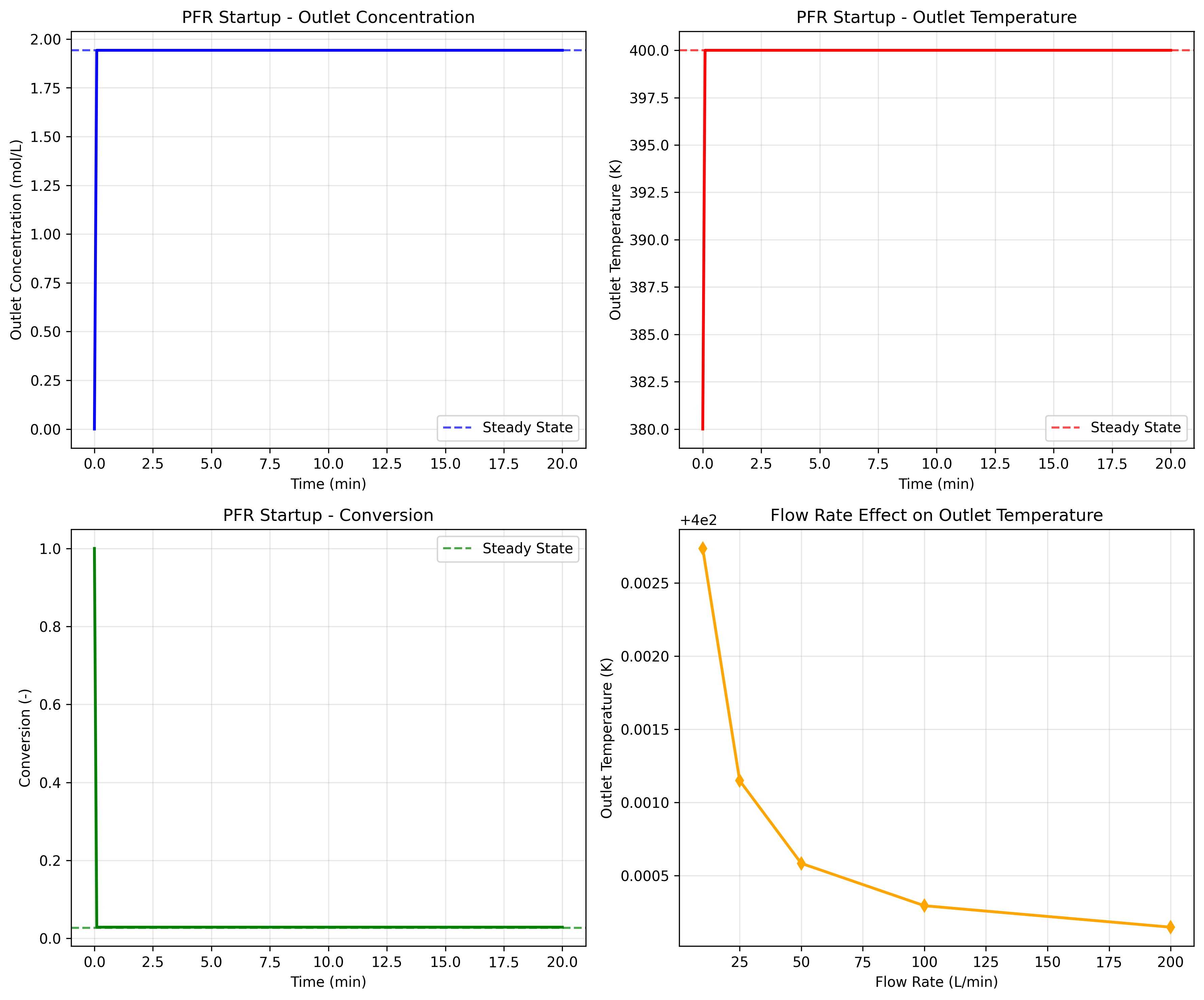
Dynamic Response (plug_flow_reactor_detailed_analysis.png)

Applications

• Tubular reactors in petrochemical industry

• Gas-phase high-temperature reactions

• Steam cracking and reforming

• Catalytic processes in tubes

• Continuous polymerization

Example Output

Running the complete example produces the following results:

============================================================
PlugFlowReactor (PFR) Example
============================================================
Reactor: Example_PFR
Length: 10.0 m
Cross-sectional area: 0.1 m²
Number of segments: 20
Segment length: 0.500 m

Operating Conditions:
  q: 50.0 L/min
  CAi: 2.0 mol/L
  Ti: 400.0 K
  Tw: 380.0 K

Steady-State Analysis:
------------------------------
Overall conversion: 2.7%
Inlet concentration: 1.997 mol/L
Outlet concentration: 1.942 mol/L
Inlet temperature: 400.0 K
Outlet temperature: 400.0 K
Maximum temperature: 400.0 K
Residence time: 0.02 min
Superficial velocity: 0.0083 m/s

Performance Plots

The example generates visualization files:

Axial Profiles (plug_flow_reactor_example_plots.png)

Shows concentration and temperature evolution along reactor length.

Detailed Analysis (plug_flow_reactor_detailed_analysis.png)

Shows parametric studies of flow rate and wall temperature effects.

Limitations

• No radial mixing assumed

• Single reaction kinetics

• Constant physical properties

• Steady axial flow assumption

Literature References

1. Fogler, H.S. (2016). Elements of Chemical Reaction Engineering, 5th Edition, Prentice Hall.

2. Levenspiel, O. (1999). Chemical Reaction Engineering, 3rd Edition, John Wiley & Sons.

3. Froment, G.F., Bischoff, K.B., and De Wilde, J. (2010). Chemical Reactor Analysis and Design, 3rd Edition, John Wiley & Sons.

See Also

• Continuous Stirred Tank Reactor (CSTR) - Continuous stirred tank reactor

• Fixed Bed Reactor - Fixed bed catalytic reactor