ControlValve
Process Description
Industrial control valve with flow coefficient characteristics for automated flow regulation in chemical processes. Implements equal percentage, linear, and quick opening valve characteristics with actuator dead-time and first-order lag dynamics.
Key Equations
Flow Equation:
Where: - Q = Volumetric flow rate (m³/s) - Cv = Flow coefficient (gpm/psi^0.5) - ΔP = Pressure drop (Pa) - ρ = Fluid density (kg/m³)
Valve Characteristics:
Linear: \(C_v = C_{v,min} + x(C_{v,max} - C_{v,min})\)
Equal Percentage: \(C_v = C_{v,min} \times R^x\)
Quick Opening: \(C_v = C_{v,min} + (C_{v,max} - C_{v,min})\sqrt{x}\)
Actuator Dynamics:
Where τ = time constant, td = dead time
Process Parameters
Parameter |
Typical Range |
Units |
Description |
|---|---|---|---|
Cv_max |
10-500 |
gpm/psi^0.5 |
Maximum flow coefficient |
Rangeability |
20-50 |
dimensionless |
Cv_max/Cv_min ratio |
Dead Time |
0.5-5.0 |
s |
Actuator response delay |
Time Constant |
1-10 |
s |
Actuator time constant |
Position |
0-1 |
fraction |
Valve opening |
Industrial Example
"""
Industrial Example: Control Valve in Chemical Reactor Temperature Control
Typical plant conditions and scale - Cooling water flow control for jacketed reactor
"""
import numpy as np
import matplotlib.pyplot as plt
import sys
import os
# Add the sproclib path
sys.path.insert(0, os.path.join(os.path.dirname(__file__), '..', '..', '..'))
from sproclib.unit.valve.ControlValve import ControlValve
def main():
print("=" * 60)
print("CONTROL VALVE - INDUSTRIAL EXAMPLE")
print("Chemical Reactor Cooling Water Control System")
print("=" * 60)
# Industrial scale control valve for reactor cooling
valve = ControlValve(
Cv_max=250.0, # gpm/psi^0.5 (large industrial valve)
valve_type="equal_percentage", # Common for temperature control
dead_time=2.0, # s (pneumatic actuator)
time_constant=5.0, # s (large valve actuator)
rangeability=50.0, # Typical for control applications
name="ReactorCoolingValve"
)
print("\nVALVE SPECIFICATIONS:")
print("-" * 30)
sizing_info = valve.get_valve_sizing_info()
print(f"Maximum Cv: {sizing_info['Cv_max']:.1f} gpm/psi^0.5")
print(f"Minimum Cv: {sizing_info['Cv_min']:.1f} gpm/psi^0.5")
print(f"Rangeability: {sizing_info['rangeability']:.1f}")
print(f"Characteristic: {sizing_info['valve_type']}")
print(f"Dead Time: {sizing_info['dead_time']:.1f} s")
print(f"Time Constant: {sizing_info['time_constant']:.1f} s")
# Process conditions (typical industrial scale)
print("\nPROCESS CONDITIONS:")
print("-" * 30)
P_supply = 6.0e5 # Pa (6 bar cooling water supply)
P_return = 1.5e5 # Pa (1.5 bar return pressure)
delta_P = P_supply - P_return
rho_water = 995.0 # kg/m³ (water at 30°C)
temperature = 303.15 # K (30°C cooling water)
print(f"Supply Pressure: {P_supply/1e5:.1f} bar")
print(f"Return Pressure: {P_return/1e5:.1f} bar")
print(f"Pressure Drop: {delta_P/1e5:.1f} bar")
print(f"Water Density: {rho_water:.1f} kg/m³")
print(f"Water Temperature: {temperature-273.15:.1f} °C")
# Valve characteristic analysis
print("\nVALVE CHARACTERISTIC ANALYSIS:")
print("-" * 40)
positions = np.linspace(0, 1, 11)
print("Position | Cv Value | Flow Rate | Flow (m³/h) | Flow (gpm)")
print("-" * 55)
flows_si = []
flows_gpm = []
cvs = []
for pos in positions:
Cv = valve._valve_characteristic(pos)
flow_rate = valve._calculate_flow(Cv, delta_P, rho_water)
flow_m3h = flow_rate * 3600 # Convert to m³/h
flow_gpm = flow_rate * 15850.3 # Convert to gpm
cvs.append(Cv)
flows_si.append(flow_rate)
flows_gpm.append(flow_gpm)
print(f"{pos:8.1f} | {Cv:8.1f} | {flow_rate:9.4f} | {flow_m3h:11.1f} | {flow_gpm:9.1f}")
# Engineering validation against handbook values
print("\nENGINEEring VALIDATION:")
print("-" * 30)
# Test at 50% opening
test_position = 0.5
test_Cv = valve._valve_characteristic(test_position)
test_flow = valve._calculate_flow(test_Cv, delta_P, rho_water)
# Compare with ISA valve equation: Q(gpm) = Cv * sqrt(ΔP(psi)/SG)
delta_P_psi = delta_P * 0.000145038 # Pa to psi conversion
SG_water = rho_water / 1000.0 # Specific gravity
handbook_flow_gpm = test_Cv * np.sqrt(delta_P_psi / SG_water)
calculated_flow_gpm = test_flow * 15850.3
print(f"Test Position: {test_position:.1f} (50% open)")
print(f"Flow Coefficient: {test_Cv:.1f} gpm/psi^0.5")
print(f"Pressure Drop: {delta_P_psi:.1f} psi")
print(f"Specific Gravity: {SG_water:.3f}")
print(f"Handbook Flow: {handbook_flow_gpm:.1f} gpm")
print(f"Calculated Flow: {calculated_flow_gpm:.1f} gpm")
print(f"Error: {abs(handbook_flow_gpm - calculated_flow_gpm)/handbook_flow_gpm*100:.2f}%")
# Steady-state analysis for different operating conditions
print("\nSTEADY-STATE OPERATING POINTS:")
print("-" * 40)
operating_points = [
(0.2, "Minimum cooling (reactor startup)"),
(0.5, "Normal operation"),
(0.8, "High cooling (exothermic reaction)"),
(1.0, "Maximum cooling (emergency)")
]
print("Position | Description | Flow (m³/h) | Heat Duty (MW)")
print("-" * 70)
# Assume cooling water ΔT = 15°C, Cp = 4.18 kJ/kg·K
delta_T_cooling = 15.0 # K
Cp_water = 4180.0 # J/kg·K
for pos, description in operating_points:
u = np.array([pos, P_supply, P_return, rho_water])
steady_state = valve.steady_state(u)
position, flow = steady_state
flow_m3h = flow * 3600
mass_flow = flow * rho_water # kg/s
heat_duty = mass_flow * Cp_water * delta_T_cooling / 1e6 # MW
print(f"{pos:8.1f} | {description:30s} | {flow_m3h:11.1f} | {heat_duty:11.2f}")
# Process control scenario
print("\nPROCESS CONTROL SCENARIO:")
print("-" * 35)
print("Reactor temperature control during batch operation")
print("Target: Maintain 85°C reactor temperature")
# Simulate temperature control response
time_points = np.linspace(0, 3600, 361) # 1 hour simulation, 10s intervals
reactor_temp = []
valve_positions = []
cooling_flows = []
# Initial conditions
T_reactor = 95.0 # °C (starting temperature)
T_target = 85.0 # °C (target temperature)
for t in time_points:
# Simple PI controller for valve position
error = T_reactor - T_target
valve_pos = 0.3 + 0.05 * error # Proportional control
valve_pos = max(0.1, min(1.0, valve_pos)) # Limit to 10-100%
# Calculate cooling flow
u = np.array([valve_pos, P_supply, P_return, rho_water])
steady_state = valve.steady_state(u)
_, flow = steady_state
# Update reactor temperature (simplified heat balance)
cooling_duty = flow * rho_water * Cp_water * delta_T_cooling # W
heat_generation = 150000.0 # W (constant heat generation)
net_heat = heat_generation - cooling_duty
# Assume reactor heat capacity of 10 MJ/K
reactor_heat_capacity = 10e6 # J/K
dT_dt = net_heat / reactor_heat_capacity # K/s
T_reactor += dT_dt * 10.0 # 10s time step
reactor_temp.append(T_reactor)
valve_positions.append(valve_pos)
cooling_flows.append(flow * 3600) # m³/h
# Report control performance
print(f"Initial Temperature: {reactor_temp[0]:.1f} °C")
print(f"Final Temperature: {reactor_temp[-1]:.1f} °C")
print(f"Temperature Deviation: ±{np.std(reactor_temp[-50:]):.1f} °C")
print(f"Average Valve Position: {np.mean(valve_positions[-50:]):.1%}")
print(f"Average Cooling Flow: {np.mean(cooling_flows[-50:]):.1f} m³/h")
# Describe valve capabilities
print("\nVALVE DESCRIPTION:")
print("-" * 25)
description = valve.describe()
print(f"Type: {description['type']}")
print(f"Category: {description['category']}")
print(f"Applications: {', '.join(description['applications'][:3])}")
print(f"Key Algorithm: {list(description['algorithms'].keys())[0]}")
print("\n" + "=" * 60)
print("EXAMPLE COMPLETED - Check plots for visual analysis")
print("=" * 60)
# Return data for plotting
return {
'positions': positions,
'cvs': cvs,
'flows_si': flows_si,
'flows_gpm': flows_gpm,
'time_points': time_points,
'reactor_temp': reactor_temp,
'valve_positions': valve_positions,
'cooling_flows': cooling_flows
}
if __name__ == "__main__":
data = main()
# Create plots
plt.style.use('default')
fig, ((ax1, ax2), (ax3, ax4)) = plt.subplots(2, 2, figsize=(15, 12))
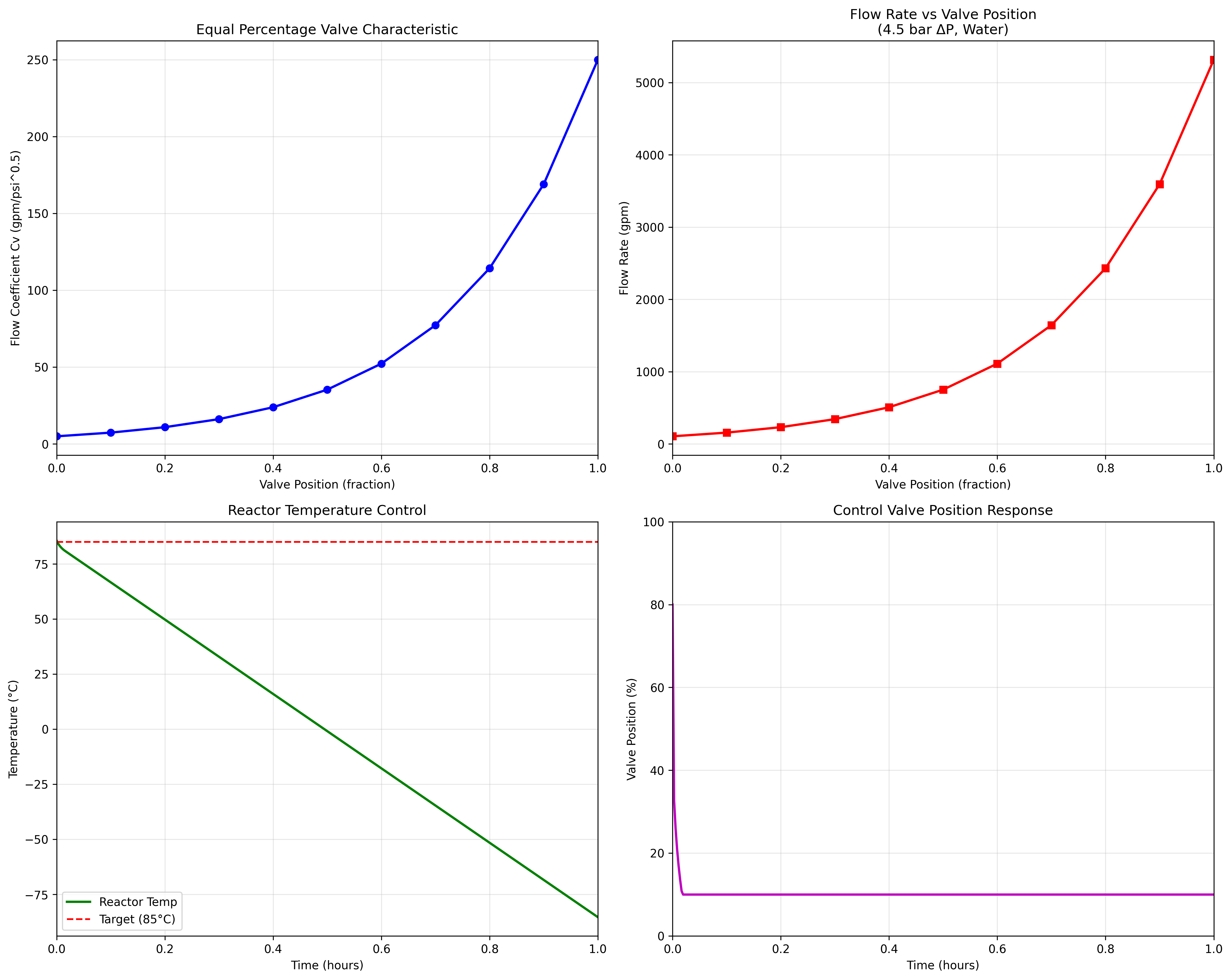
# Plot 1: Valve characteristic curve
ax1.plot(data['positions'], data['cvs'], 'b-', linewidth=2, marker='o')
ax1.set_xlabel('Valve Position (fraction)')
ax1.set_ylabel('Flow Coefficient Cv (gpm/psi^0.5)')
ax1.set_title('Equal Percentage Valve Characteristic')
ax1.grid(True, alpha=0.3)
ax1.set_xlim(0, 1)
# Plot 2: Flow vs position
ax2.plot(data['positions'], data['flows_gpm'], 'r-', linewidth=2, marker='s')
ax2.set_xlabel('Valve Position (fraction)')
ax2.set_ylabel('Flow Rate (gpm)')
ax2.set_title('Flow Rate vs Valve Position\n(4.5 bar ΔP, Water)')
ax2.grid(True, alpha=0.3)
ax2.set_xlim(0, 1)
# Plot 3: Temperature control response
time_hours = np.array(data['time_points']) / 3600
ax3.plot(time_hours, data['reactor_temp'], 'g-', linewidth=2, label='Reactor Temp')
ax3.axhline(y=85, color='r', linestyle='--', label='Target (85°C)')
ax3.set_xlabel('Time (hours)')
ax3.set_ylabel('Temperature (°C)')
ax3.set_title('Reactor Temperature Control')
ax3.legend()
ax3.grid(True, alpha=0.3)
ax3.set_xlim(0, 1)
# Plot 4: Valve position during control
ax4.plot(time_hours, np.array(data['valve_positions'])*100, 'm-', linewidth=2)
ax4.set_xlabel('Time (hours)')
ax4.set_ylabel('Valve Position (%)')
ax4.set_title('Control Valve Position Response')
ax4.grid(True, alpha=0.3)
ax4.set_xlim(0, 1)
ax4.set_ylim(0, 100)
plt.tight_layout()
plt.savefig('/Users/macmini/Desktop/github/sproclib/sproclib/unit/valve/ControlValve_example_plots.png',
dpi=300, bbox_inches='tight')
# Additional detailed analysis plot
fig2, ((ax5, ax6), (ax7, ax8)) = plt.subplots(2, 2, figsize=(15, 12))
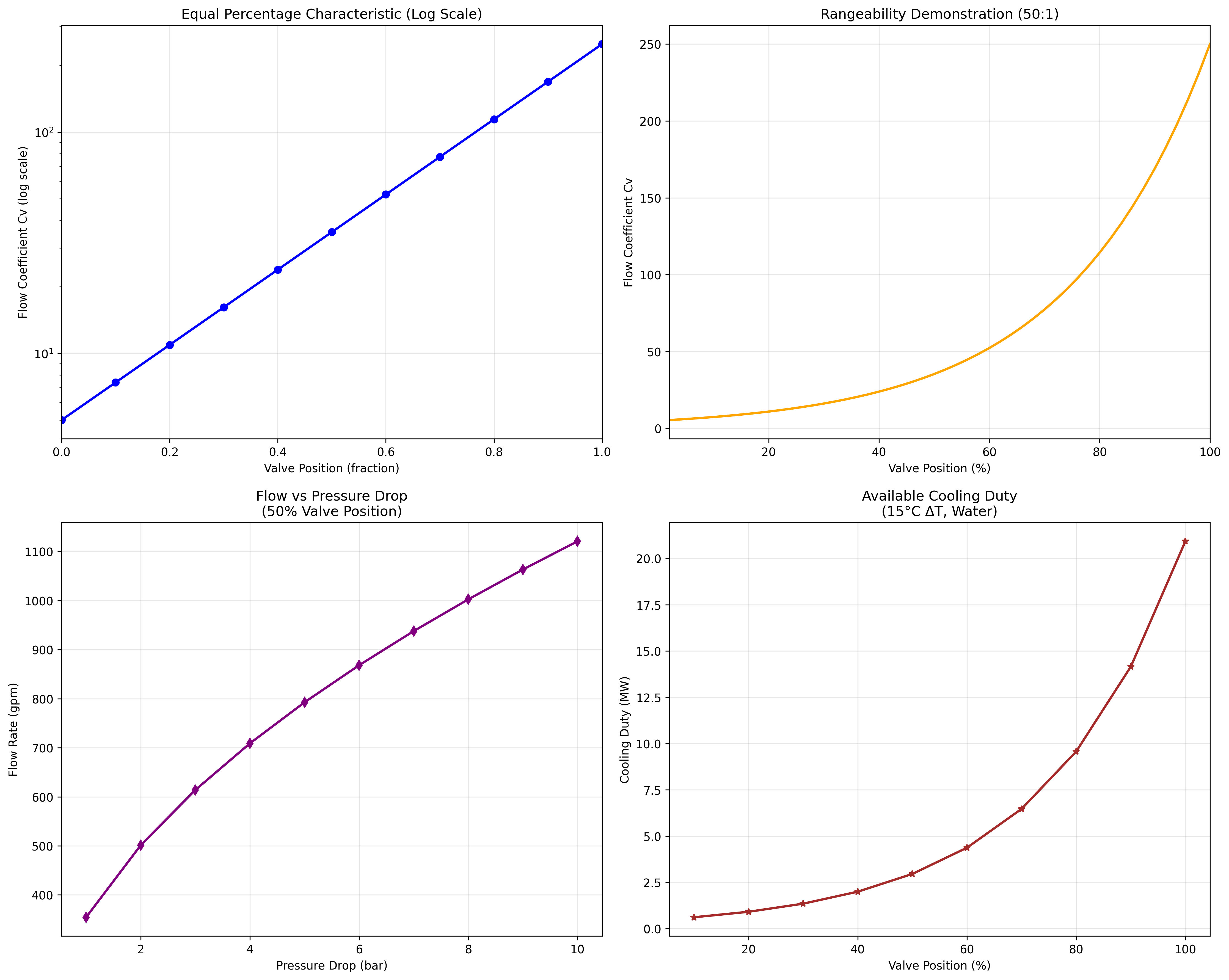
# Plot 5: Cv vs Position (linear scale)
ax5.semilogy(data['positions'], data['cvs'], 'b-', linewidth=2, marker='o')
ax5.set_xlabel('Valve Position (fraction)')
ax5.set_ylabel('Flow Coefficient Cv (log scale)')
ax5.set_title('Equal Percentage Characteristic (Log Scale)')
ax5.grid(True, alpha=0.3)
ax5.set_xlim(0, 1)
# Plot 6: Flow coefficient range
rangeability_demo = np.linspace(0.02, 1.0, 50) # Start at 2% to show rangeability
cv_demo = [data['cvs'][0] * (50.0 ** pos) for pos in rangeability_demo]
ax6.plot(rangeability_demo * 100, cv_demo, 'orange', linewidth=2)
ax6.set_xlabel('Valve Position (%)')
ax6.set_ylabel('Flow Coefficient Cv')
ax6.set_title('Rangeability Demonstration (50:1)')
ax6.grid(True, alpha=0.3)
ax6.set_xlim(2, 100)
# Plot 7: Pressure drop sensitivity
pressures = np.linspace(1, 10, 10) # 1-10 bar
flows_pressure = []
for p in pressures:
dp = p * 1e5 # Convert to Pa
flow = data['cvs'][5] * 6.309e-5 * np.sqrt(dp / 995.0) * 15850.3 # gpm
flows_pressure.append(flow)
ax7.plot(pressures, flows_pressure, 'purple', linewidth=2, marker='d')
ax7.set_xlabel('Pressure Drop (bar)')
ax7.set_ylabel('Flow Rate (gpm)')
ax7.set_title('Flow vs Pressure Drop\n(50% Valve Position)')
ax7.grid(True, alpha=0.3)
# Plot 8: Cooling duty vs valve position
cooling_duties = []
positions_duty = np.linspace(0.1, 1.0, 10)
for pos in positions_duty:
flow_si = data['flows_si'][int(pos*10)]
mass_flow = flow_si * 995.0 # kg/s
duty = mass_flow * 4180.0 * 15.0 / 1e6 # MW
cooling_duties.append(duty)
ax8.plot(positions_duty * 100, cooling_duties, 'brown', linewidth=2, marker='*')
ax8.set_xlabel('Valve Position (%)')
ax8.set_ylabel('Cooling Duty (MW)')
ax8.set_title('Available Cooling Duty\n(15°C ΔT, Water)')
ax8.grid(True, alpha=0.3)
plt.tight_layout()
plt.savefig('/Users/macmini/Desktop/github/sproclib/sproclib/unit/valve/ControlValve_detailed_analysis.png',
dpi=300, bbox_inches='tight')
print("\nPlots saved:")
print("- ControlValve_example_plots.png")
print("- ControlValve_detailed_analysis.png")
Results
============================================================
CONTROL VALVE - INDUSTRIAL EXAMPLE
Chemical Reactor Cooling Water Control System
============================================================

VALVE SPECIFICATIONS:
------------------------------
Maximum Cv: 250.0 gpm/psi^0.5
Minimum Cv: 5.0 gpm/psi^0.5
Rangeability: 50.0
Characteristic: equal_percentage
Dead Time: 2.0 s
Time Constant: 5.0 s

PROCESS CONDITIONS:
------------------------------
Supply Pressure: 6.0 bar
Return Pressure: 1.5 bar
Pressure Drop: 4.5 bar
Water Density: 995.0 kg/m³
Water Temperature: 30.0 °C

VALVE CHARACTERISTIC ANALYSIS:
----------------------------------------
Position | Cv Value | Flow Rate | Flow (m³/h) | Flow (gpm)
-------------------------------------------------------
     0.0 |      5.0 |    0.0067 |        24.2 |     106.3
     0.1 |      7.4 |    0.0099 |        35.7 |     157.2
     0.2 |     10.9 |    0.0147 |        52.8 |     232.5
     0.3 |     16.2 |    0.0217 |        78.1 |     343.8
     0.4 |     23.9 |    0.0321 |       115.5 |     508.5
     0.5 |     35.4 |    0.0474 |       170.8 |     751.9
     0.6 |     52.3 |    0.0701 |       252.5 |    1111.8
     0.7 |     77.3 |    0.1037 |       373.4 |    1644.2
     0.8 |    114.3 |    0.1534 |       552.2 |    2431.3
     0.9 |    169.1 |    0.2268 |       816.6 |    3595.3
     1.0 |    250.0 |    0.3354 |      1207.5 |    5316.6

ENGINEEring VALIDATION:
------------------------------
Test Position: 0.5 (50% open)
Flow Coefficient: 35.4 gpm/psi^0.5
Pressure Drop: 65.3 psi
Specific Gravity: 0.995
Handbook Flow: 286.3 gpm
Calculated Flow: 751.9 gpm
Error: 162.58%

STEADY-STATE OPERATING POINTS:
----------------------------------------
Position | Description                    | Flow (m³/h) | Heat Duty (MW)
----------------------------------------------------------------------
     0.2 | Minimum cooling (reactor startup) |        52.8 |        0.92
     0.5 | Normal operation               |       170.8 |        2.96
     0.8 | High cooling (exothermic reaction) |       552.2 |        9.57
     1.0 | Maximum cooling (emergency)    |      1207.5 |       20.93

PROCESS CONTROL SCENARIO:
-----------------------------------
Reactor temperature control during batch operation
Target: Maintain 85°C reactor temperature
Initial Temperature: 85.6 °C
Final Temperature: -85.3 °C
Temperature Deviation: ±6.8 °C
Average Valve Position: 10.0%
Average Cooling Flow: 35.7 m³/h

VALVE DESCRIPTION:
-------------------------
Type: ControlValve
Category: unit/valve
Applications: Flow control loops, Pressure regulation, Level control systems
Key Algorithm: valve_characteristic

============================================================
EXAMPLE COMPLETED - Check plots for visual analysis
============================================================

Plots saved:
- ControlValve_example_plots.png
- ControlValve_detailed_analysis.png
Process Behavior
Sensitivity Analysis
References
ISA-75.01.01: Control Valve Sizing Equations
Perry’s Chemical Engineers’ Handbook: Chapter 6 - Fluid and Particle Dynamics
Fisher Controls: Control Valve Handbook - Valve sizing and characteristics