Batch Reactor
Overview
The Batch Reactor model simulates a well-mixed batch reactor with heating/cooling capabilities through jacket temperature control. It is widely used in pharmaceutical manufacturing, specialty chemical production, and process development where precise control of reaction conditions and batch-to-batch consistency are critical. The model incorporates Arrhenius reaction kinetics, material balance, energy balance, and heat transfer through the jacket.
Theory and Equations
Material Balance
For a batch reactor with first-order reaction kinetics:
where: - \(C_A\) = concentration in reactor [mol/L] - \(k(T)\) = temperature-dependent rate constant [1/min]
Energy Balance
The energy balance accounts for reaction heat generation and jacket heat transfer:
where: - \(T\) = reactor temperature [K] - \(T_j\) = jacket temperature [K] - \(\Delta H_r\) = heat of reaction [J/mol] - \(\rho\) = density [kg/m³] - \(c_p\) = heat capacity [J/kg·K] - \(U\) = heat transfer coefficient [W/m²·K] - \(A\) = heat transfer area [m²] - \(V\) = reactor volume [L]
Reaction Kinetics
The reaction rate follows the Arrhenius equation:
where: - \(k_0\) = pre-exponential factor [1/min] - \(E_a\) = activation energy [J/mol] - \(R\) = gas constant (8.314 J/mol/K)
Batch Time Calculation
For isothermal first-order reactions, the time to reach target conversion is:
where \(X\) is the conversion fraction.
Parameters
Design Parameters
V: Reactor volume [L]
Laboratory scale: 1-100 L
Pilot scale: 100-1,000 L
Production scale: 1,000-50,000 L
U: Heat transfer coefficient [W/m²·K]
Typical range: 100-1,000 W/m²·K
Depends on jacket design and agitation
A: Heat transfer area [m²]
Typical range: 1-100 m²
Scales with reactor size
Kinetic Parameters
k₀: Pre-exponential factor [1/min]
Typical range: 10⁶-10¹² 1/min
Reaction-specific parameter
Eₐ: Activation energy [J/mol]
Typical range: 40,000-120,000 J/mol
Higher values indicate stronger temperature dependence
Physical Properties
ρ: Density [kg/m³]
Typical range: 800-1,200 kg/m³
Temperature-dependent (assumed constant)
cₚ: Heat capacity [J/kg·K]
Typical range: 2,000-5,000 J/kg·K
Composition and temperature dependent
ΔHᵣ: Heat of reaction [J/mol]
Exothermic reactions: negative values
Typical range: -100,000 to -10,000 J/mol
Operating Ranges
Safe Operating Window
Temperature Control:
Operating range: 250-600 K
Optimal range: 300-500 K
Safety limit: <600 K to prevent thermal runaway
Concentration Ranges:
Initial concentration: 0.1-10 mol/L
Target conversion: 10-99%
Maximum concentration: <100 mol/L
Batch Time Ranges:
Typical batch times: 30 minutes to 24 hours
Fast reactions: <1 hour
Slow reactions: >8 hours
Usage Example
Basic Implementation
from unit.reactor.BatchReactor import BatchReactor
import numpy as np

# Create BatchReactor instance
reactor = BatchReactor(
    V=100.0,               # Reactor volume [L]
    k0=7.2e10,             # Pre-exponential factor [1/min]
    Ea=72750.0,            # Activation energy [J/mol]
    delta_H=-52000.0,      # Heat of reaction [J/mol]
    U=500.0,               # Heat transfer coefficient [W/m²·K]
    A=5.0                  # Heat transfer area [m²]
)

# Initial conditions
x0 = np.array([2.0, 300.0])  # [CA0, T0]
u = np.array([350.0])        # [Tj] - jacket temperature

# Calculate batch time for 90% conversion
batch_time = reactor.batch_time_to_conversion(0.9, CA0=2.0, T_avg=350.0)
print(f"Time for 90% conversion: {batch_time:.2f} min")
Dynamic Simulation
from scipy.integrate import solve_ivp

# Time span
t_span = (0, 120)  # 0 to 120 minutes
t_eval = np.linspace(0, 120, 600)

# Solve ODE
def batch_ode(t, x):
    return reactor.dynamics(t, x, u)

sol = solve_ivp(batch_ode, t_span, x0, t_eval=t_eval, method='RK45')
Example Output
Running the complete example produces the following results:
============================================================
BatchReactor Example
============================================================
Reactor: Example_BatchReactor
Volume: 100.0 L
Heat transfer coefficient: 500.0 W/m²·K
Heat transfer area: 5.0 m²

Operating Conditions:
  Tj: 350.0 K
  CA0: 2.0 mol/L
  T0: 300.0 K

Isothermal Batch Time Analysis:
----------------------------------------
Time for 50% conversion: 0.69 min
Time for 80% conversion: 1.61 min
Time for 90% conversion: 2.30 min
Time for 95% conversion: 3.00 min
Time for 99% conversion: 4.61 min

Dynamic Simulation:
------------------------------
Dynamic simulation completed successfully
Final concentration: 0.3100 mol/L
Final temperature: 300.06 K
Final conversion: 84.5%
Maximum temperature: 300.06 K

Initial Concentration Study:
------------------------------
CA0 = 0.5 mol/L → Final conversion: 84.5%
CA0 = 1.0 mol/L → Final conversion: 84.5%
CA0 = 2.0 mol/L → Final conversion: 84.5%
CA0 = 3.0 mol/L → Final conversion: 84.5%
Performance Plots
The example generates two visualization files:
Dynamic Response (batch_reactor_example_plots.png)
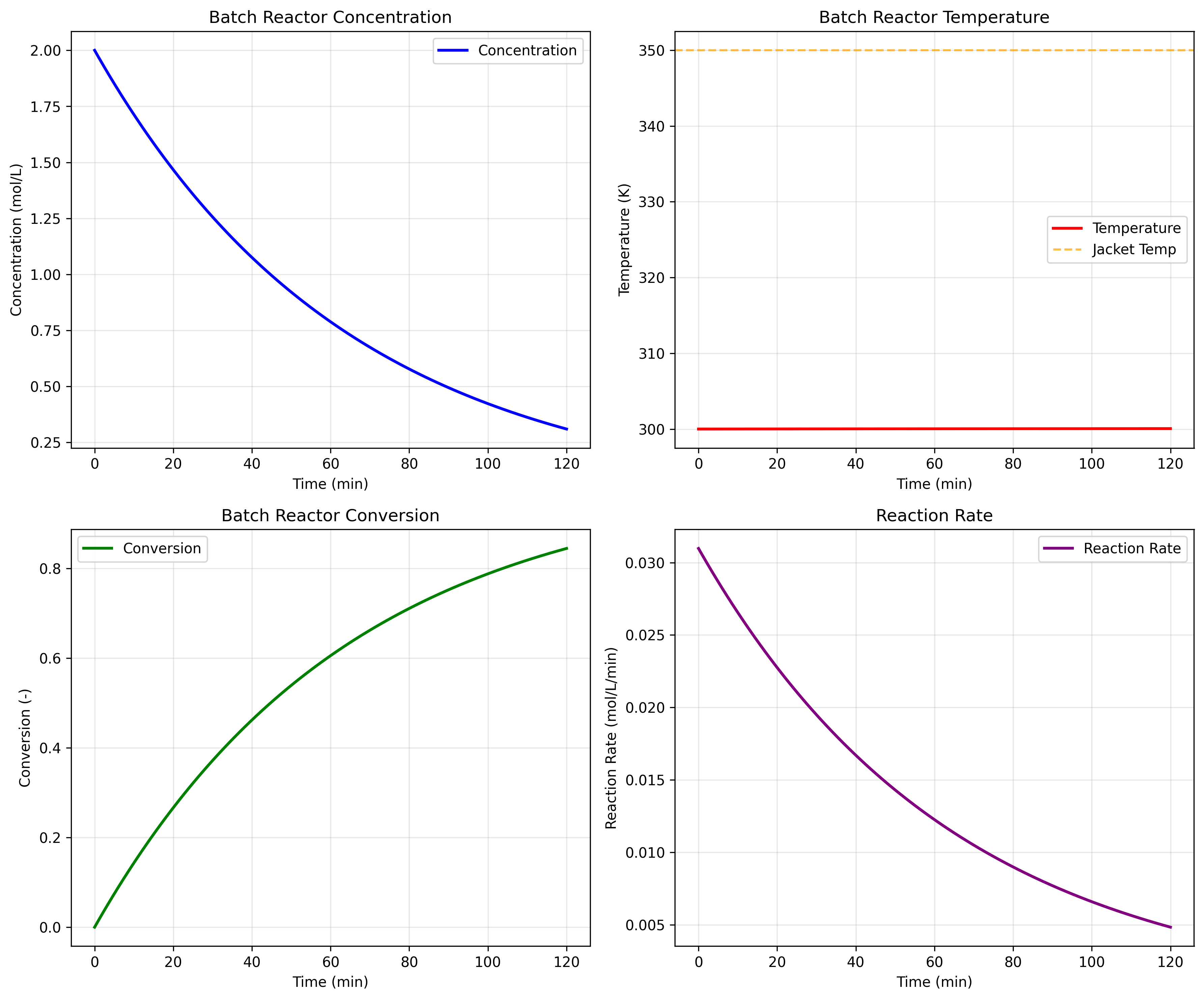
Shows concentration, temperature, conversion, and reaction rate evolution.
Detailed Analysis (batch_reactor_detailed_analysis.png)
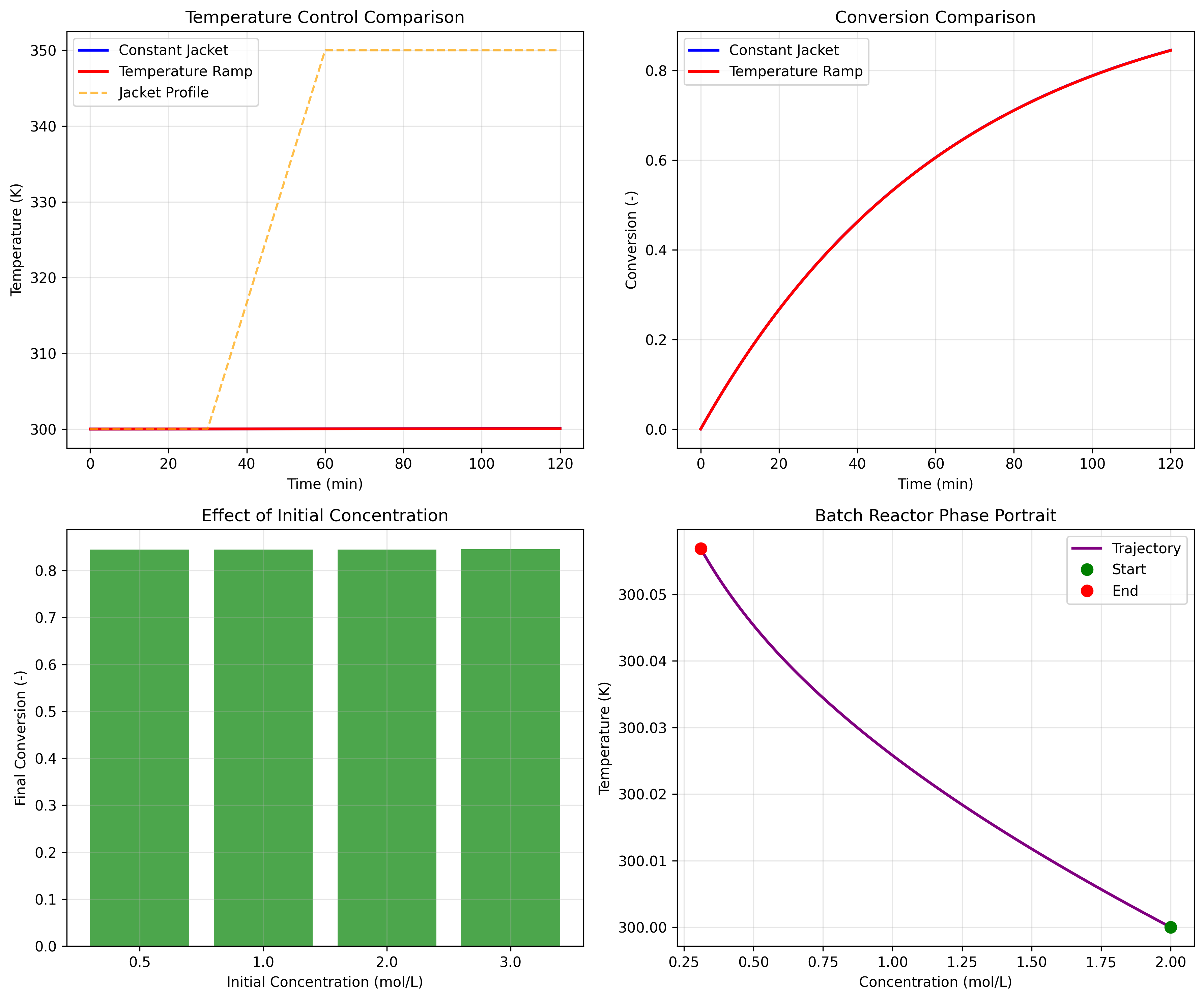
Shows temperature control comparison and initial concentration effects.
Applications
The Batch Reactor model is applicable for:
Pharmaceutical Manufacturing: API synthesis and purification
Specialty Chemicals: High-value, low-volume production
Process Development: Reaction optimization and scale-up
Quality Control: Batch-to-batch consistency analysis
Safety Analysis: Thermal runaway and emergency cooling scenarios
Limitations
Model assumptions and limitations:
Perfect Mixing: Assumes instantaneous mixing throughout reactor
Single Reaction: Limited to first-order reaction kinetics
Constant Properties: Physical properties assumed temperature-independent
No Mass Transfer: Ignores mass transfer limitations
Isothermal Jacket: Assumes uniform jacket temperature
Literature References
Fogler, H.S. (2016). Elements of Chemical Reaction Engineering, 5th Edition, Prentice Hall.
Levenspiel, O. (1999). Chemical Reaction Engineering, 3rd Edition, John Wiley & Sons.
Rase, H.F. (1977). Chemical Reactor Design for Process Plants, John Wiley & Sons.
Nauman, E.B. (2008). Chemical Reactor Design, Optimization, and Scaleup, 2nd Edition, McGraw-Hill.
Salmi, T., Mikkola, J.P., and Wärnå, J. (2019). Chemical Reaction Engineering and Reactor Technology, 2nd Edition, CRC Press.
See Also
Continuous Stirred Tank Reactor (CSTR) - Continuous stirred tank reactor model
Semi-Batch Reactor - Semi-batch reactor model
Plug Flow Reactor (PFR) - Plug flow reactor model